7 Discriminant Analysis

Discriminant Analysis의 장점

고차원의 데이터셋을 관리가 훨씬 쉬운 저차원으로 축소하여 예측을 수행한다.
차원축소를 통해 얻은 판별점수는 다른 분류 예측 알고리듬의 예측 변수로 활용 가능하다.
정규성을 만족할 경우, 로지스틱 회귀분석보다 더 효과적이다.
- 30% 정도 더 효과적인 성능을 발휘한다.
데이터셋의 크기가 작을 때 유용하게 적용할 수 있다.

Discriminant Analysis의 단점

연속형 예측 변수만 가능하다.

실습 자료 : 1912년 4월 15일 타이타닉호 침몰 당시 탑승객들의 정보를 기록한 데이터셋이며, 총 11개의 변수를 포함하고 있다. 이 자료에서 Target은 Survived이다.

7.1 데이터 불러오기

pacman::p_load("data.table", 
               "tidyverse", 
               "dplyr", "tidyr",
               "caret",
               "ggplot2", "GGally",
               "biotools",                 # For boxM
               "MASS",                     # For lda and qda
               "DescTools",                # For Desc
               "klaR"                      # For partimat
               )

titanic <- fread("../Titanic.csv")                                      # 데이터 불러오기

titanic %>%
  as_tibble

# A tibble: 891 × 11
   Survived Pclass Name                                                Sex      Age SibSp Parch Ticket            Fare Cabin  Embarked
      <int>  <int> <chr>                                               <chr>  <dbl> <int> <int> <chr>            <dbl> <chr>  <chr>   
 1        0      3 Braund, Mr. Owen Harris                             male      22     1     0 A/5 21171         7.25 ""     S       
 2        1      1 Cumings, Mrs. John Bradley (Florence Briggs Thayer) female    38     1     0 PC 17599         71.3  "C85"  C       
 3        1      3 Heikkinen, Miss. Laina                              female    26     0     0 STON/O2. 3101282  7.92 ""     S       
 4        1      1 Futrelle, Mrs. Jacques Heath (Lily May Peel)        female    35     1     0 113803           53.1  "C123" S       
 5        0      3 Allen, Mr. William Henry                            male      35     0     0 373450            8.05 ""     S       
 6        0      3 Moran, Mr. James                                    male      NA     0     0 330877            8.46 ""     Q       
 7        0      1 McCarthy, Mr. Timothy J                             male      54     0     0 17463            51.9  "E46"  S       
 8        0      3 Palsson, Master. Gosta Leonard                      male       2     3     1 349909           21.1  ""     S       
 9        1      3 Johnson, Mrs. Oscar W (Elisabeth Vilhelmina Berg)   female    27     0     2 347742           11.1  ""     S       
10        1      2 Nasser, Mrs. Nicholas (Adele Achem)                 female    14     1     0 237736           30.1  ""     C       
# ℹ 881 more rows

7.2 데이터 전처리 I

titanic %<>%
  data.frame() %>%                                                      # Data Frame 형태로 변환 
  mutate(Survived = ifelse(Survived == 1, "yes", "no"))                 # Target을 문자형 변수로 변환

# 1. Convert to Factor
titanic$Survived <- factor(titanic$Survived)                            # Target을 범주형으로 변환

# 2. Generate New Variable
titanic <- titanic %>%
  mutate(FamSize = SibSp + Parch)                                       # "FamSize = 형제 및 배우자 수 + 부모님 및 자녀 수"로 가족 수를 의미하는 새로운 변수

glimpse(titanic)                                                        # 데이터 구조 확인

Rows: 891
Columns: 12
$ Survived <fct> no, yes, yes, yes, no, no, no, no, yes, yes, yes, yes, no, no, no, yes, no, yes, no, yes, no, yes, yes, yes, no, yes, no, no, yes, no, no, yes, yes, no, no, no, yes, no, no, yes, no…
$ Pclass   <int> 3, 1, 3, 1, 3, 3, 1, 3, 3, 2, 3, 1, 3, 3, 3, 2, 3, 2, 3, 3, 2, 2, 3, 1, 3, 3, 3, 1, 3, 3, 1, 1, 3, 2, 1, 1, 3, 3, 3, 3, 3, 2, 3, 2, 3, 3, 3, 3, 3, 3, 3, 3, 1, 2, 1, 1, 2, 3, 2, 3, 3…
$ Name     <chr> "Braund, Mr. Owen Harris", "Cumings, Mrs. John Bradley (Florence Briggs Thayer)", "Heikkinen, Miss. Laina", "Futrelle, Mrs. Jacques Heath (Lily May Peel)", "Allen, Mr. William Henry…
$ Sex      <chr> "male", "female", "female", "female", "male", "male", "male", "male", "female", "female", "female", "female", "male", "male", "female", "female", "male", "male", "female", "female",…
$ Age      <dbl> 22.0, 38.0, 26.0, 35.0, 35.0, NA, 54.0, 2.0, 27.0, 14.0, 4.0, 58.0, 20.0, 39.0, 14.0, 55.0, 2.0, NA, 31.0, NA, 35.0, 34.0, 15.0, 28.0, 8.0, 38.0, NA, 19.0, NA, NA, 40.0, NA, NA, 66.…
$ SibSp    <int> 1, 1, 0, 1, 0, 0, 0, 3, 0, 1, 1, 0, 0, 1, 0, 0, 4, 0, 1, 0, 0, 0, 0, 0, 3, 1, 0, 3, 0, 0, 0, 1, 0, 0, 1, 1, 0, 0, 2, 1, 1, 1, 0, 1, 0, 0, 1, 0, 2, 1, 4, 0, 1, 1, 0, 0, 0, 0, 1, 5, 0…
$ Parch    <int> 0, 0, 0, 0, 0, 0, 0, 1, 2, 0, 1, 0, 0, 5, 0, 0, 1, 0, 0, 0, 0, 0, 0, 0, 1, 5, 0, 2, 0, 0, 0, 0, 0, 0, 0, 0, 0, 0, 0, 0, 0, 0, 0, 2, 0, 0, 0, 0, 0, 0, 1, 0, 0, 0, 1, 0, 0, 0, 2, 2, 0…
$ Ticket   <chr> "A/5 21171", "PC 17599", "STON/O2. 3101282", "113803", "373450", "330877", "17463", "349909", "347742", "237736", "PP 9549", "113783", "A/5. 2151", "347082", "350406", "248706", "38…
$ Fare     <dbl> 7.2500, 71.2833, 7.9250, 53.1000, 8.0500, 8.4583, 51.8625, 21.0750, 11.1333, 30.0708, 16.7000, 26.5500, 8.0500, 31.2750, 7.8542, 16.0000, 29.1250, 13.0000, 18.0000, 7.2250, 26.0000,…
$ Cabin    <chr> "", "C85", "", "C123", "", "", "E46", "", "", "", "G6", "C103", "", "", "", "", "", "", "", "", "", "D56", "", "A6", "", "", "", "C23 C25 C27", "", "", "", "B78", "", "", "", "", ""…
$ Embarked <chr> "S", "C", "S", "S", "S", "Q", "S", "S", "S", "C", "S", "S", "S", "S", "S", "S", "Q", "S", "S", "C", "S", "S", "Q", "S", "S", "S", "C", "S", "Q", "S", "C", "C", "Q", "S", "C", "S", "…
$ FamSize  <int> 1, 1, 0, 1, 0, 0, 0, 4, 2, 1, 2, 0, 0, 6, 0, 0, 5, 0, 1, 0, 0, 0, 0, 0, 4, 6, 0, 5, 0, 0, 0, 1, 0, 0, 1, 1, 0, 0, 2, 1, 1, 1, 0, 3, 0, 0, 1, 0, 2, 1, 5, 0, 1, 1, 1, 0, 0, 0, 3, 7, 0…

# 3. Select Variables used for Analysis
titanic1 <- titanic %>% 
  dplyr::select(Survived, Age, Fare, FamSize)                           # 분석에 사용할 변수 선택 -> 판별분석에서 예측 변수들은 다변량 정규분포를 가정하기 때문에 범주형 예측 변수는 제거

glimpse(titanic1)                                                       # 데이터 구조 확인

Rows: 891
Columns: 4
$ Survived <fct> no, yes, yes, yes, no, no, no, no, yes, yes, yes, yes, no, no, no, yes, no, yes, no, yes, no, yes, yes, yes, no, yes, no, no, yes, no, no, yes, yes, no, no, no, yes, no, no, yes, no…
$ Age      <dbl> 22.0, 38.0, 26.0, 35.0, 35.0, NA, 54.0, 2.0, 27.0, 14.0, 4.0, 58.0, 20.0, 39.0, 14.0, 55.0, 2.0, NA, 31.0, NA, 35.0, 34.0, 15.0, 28.0, 8.0, 38.0, NA, 19.0, NA, NA, 40.0, NA, NA, 66.…
$ Fare     <dbl> 7.2500, 71.2833, 7.9250, 53.1000, 8.0500, 8.4583, 51.8625, 21.0750, 11.1333, 30.0708, 16.7000, 26.5500, 8.0500, 31.2750, 7.8542, 16.0000, 29.1250, 13.0000, 18.0000, 7.2250, 26.0000,…
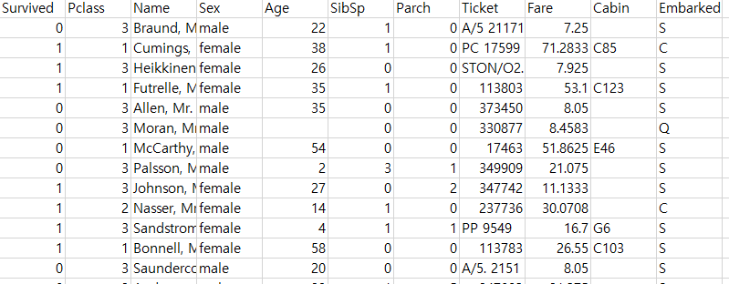
$ FamSize  <int> 1, 1, 0, 1, 0, 0, 0, 4, 2, 1, 2, 0, 0, 6, 0, 0, 5, 0, 1, 0, 0, 0, 0, 0, 4, 6, 0, 5, 0, 0, 0, 1, 0, 0, 1, 1, 0, 0, 2, 1, 1, 1, 0, 3, 0, 0, 1, 0, 2, 1, 5, 0, 1, 1, 1, 0, 0, 0, 3, 7, 0…

7.3 데이터 탐색

ggpairs(titanic1,                                        
        aes(colour = Survived)) +                         # Target의 범주에 따라 색깔을 다르게 표현
  theme_bw()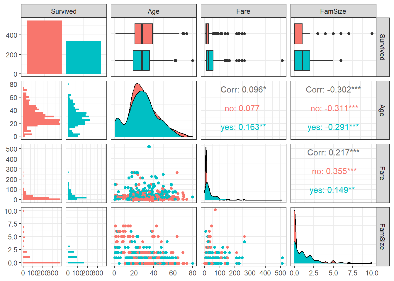

ggpairs(titanic1,                                     
        aes(colour = Survived, alpha = 0.8)) +            # Target의 범주에 따라 색깔을 다르게 표현
  scale_colour_manual(values = c("purple", "cyan4")) +    # 특정 색깔 지정
  scale_fill_manual(values = c("purple", "cyan4")) +      # 특정 색깔 지정
  theme_bw()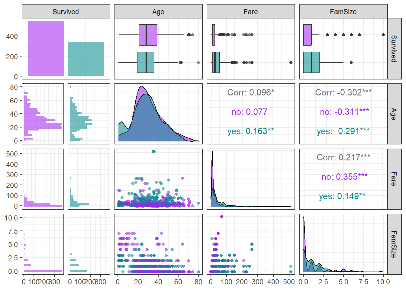

7.4 데이터 분할

# Partition (Training Dataset : Test Dataset = 7:3)
y      <- titanic1$Survived                             # Target

set.seed(200)
ind    <- createDataPartition(y, p = 0.7, list  =T)     # Index를 이용하여 7:3으로 분할
titanic.trd <- titanic1[ind$Resample1,]                 # Training Dataset
titanic.ted <- titanic1[-ind$Resample1,]                # Test Dataset

7.5 데이터 전처리 II

# 1. Imputation
titanic.trd.Imp <- titanic.trd %>% 
  mutate(Age = replace_na(Age, mean(Age, na.rm = TRUE)))                 # 평균으로 결측값 대체

titanic.ted.Imp <- titanic.ted %>% 
  mutate(Age = replace_na(Age, mean(titanic.trd$Age, na.rm = TRUE)))     # Training Dataset을 이용하여 결측값 대체

# 2. Standardization
preProcValues <- preProcess(titanic.trd.Imp, 
                            method = c("center", "scale"))               # Standardization 정의 -> Training Dataset에 대한 평균과 표준편차 계산 

titanic.trd.Imp <- predict(preProcValues, titanic.trd.Imp)               # Standardization for Training Dataset
titanic.ted.Imp <- predict(preProcValues, titanic.ted.Imp)               # Standardization for Test Dataset

glimpse(titanic.trd.Imp)                                                 # 데이터 구조 확인

Rows: 625
Columns: 4
$ Survived <fct> no, yes, yes, no, no, no, yes, yes, yes, yes, no, no, yes, no, yes, no, yes, no, no, no, yes, no, no, yes, yes, no, no, no, no, no, yes, no, no, no, yes, no, yes, no, no, no, yes, n…
$ Age      <dbl> -0.61306970, -0.30411628, 0.39102893, 0.39102893, 0.00000000, -2.15783684, -0.22687792, -1.23097656, -2.00336012, 2.16751113, 0.69998236, -1.23097656, 0.00000000, 0.08207551, 0.0000…
$ Fare     <dbl> -0.51776394, -0.50463325, 0.37414970, -0.50220165, -0.49425904, -0.24882814, -0.44222264, -0.07383411, -0.33393441, -0.14232374, -0.05040897, -0.50601052, -0.40590999, -0.30864569, …
$ FamSize  <dbl> 0.04506631, -0.55421976, 0.04506631, -0.55421976, -0.55421976, 1.84292454, 0.64435239, 0.04506631, 0.64435239, -0.55421976, 3.04149669, -0.55421976, -0.55421976, 0.04506631, -0.5542…

glimpse(titanic.ted.Imp)                                                 # 데이터 구조 확인

Rows: 266
Columns: 4
$ Survived <fct> yes, no, no, yes, no, yes, yes, yes, yes, yes, no, no, yes, yes, no, yes, no, yes, yes, no, yes, no, no, no, no, no, no, yes, yes, no, no, no, no, no, no, no, no, no, no, yes, no, n…
$ Age      <dbl> 0.62274400, 1.85855771, -0.76754642, 1.93579607, -2.15783684, 0.31379058, -1.15373820, 0.62274400, 0.00000000, -2.08059848, 0.00000000, -0.69030806, -0.07240121, -0.69030806, -0.111…
$ Fare     <dbl> 0.727866891, 0.350076786, -0.502201647, -0.347551409, -0.092232621, -0.405909990, -0.502606266, -0.048220525, -0.518168555, 0.150037190, -0.502201647, -0.507064862, -0.153022808, -0…
$ FamSize  <dbl> 0.04506631, -0.55421976, -0.55421976, -0.55421976, 2.44221062, -0.55421976, -0.55421976, 3.04149669, -0.55421976, 1.24363847, -0.55421976, -0.55421976, 0.04506631, -0.55421976, -0.5…

7.6 모공분산행렬의 동일성 검정

titanic.boxM <- boxM(titanic.trd.Imp[,-1],             # Training Dataset including Only 예측 변수 -> Target 제외
                     titanic.trd.Imp$Survived)         # Target

titanic.boxM


    Box's M-test for Homogeneity of Covariance Matrices

data:  titanic.trd.Imp[, -1]
Chi-Sq (approx.) = 269.33, df = 6, p-value < 2.2e-16

Caution! Package "biotools"에서 제공하는 함수 boxM()를 이용하여 모공분산행렬의 동일성 검정을 수행할 수 있다. 해당 검정에서 귀무가설 \(H_0\)은 “Target의 모든 클래스의 모공분산행렬은 동일하다.”이며, 귀무가설 \(H_0\)을 기각할 증거가 부족할 경우 원칙적으로는 선형판별분석을 수행한다.
Result! 가설 \(H_0 :\Sigma_{\text{yes}}=\Sigma_{\text{no}}\) vs \(H_1 :\Sigma_{\text{yes}}\ne\Sigma_{\text{no}}\)에 대하여, 카이제곱 검정통계량 \(\chi^2\)값은 269.33이며 \(p\)값은 거의 0값에 가깝다. 이에 근거하여, 유의수준 5%에서 \(p\)값이 0.05보다 작기 때문에 귀무가설 \(H_0\)를 기각할 수 있다. 즉, Training Dataset에서 Target “Survived”의 두 클래스 “no”와 “yes”의 모공분산행렬은 동일하지 않다.

7.7 선형판별분석(LDA)

7.7.1 모형 훈련

Caution! Package "MASS"에서 제공하는 함수 lda()를 통해 선형판별함수 \(L(x)\)를 얻을 수 있다. 함수 lda()는 예측 변수의 평균을 0으로 변환(중심화)한 후 분석을 수행하며, 정규화된 판별계수벡터 \(\boldsymbol{b}\)를 계산한다. 여기서, 정규화된 판별계수벡터란 합동공분산행렬을 \(\boldsymbol{S}\)라 할 때 \(\boldsymbol{b}^T \boldsymbol{S}\boldsymbol{b}=1\)을 만족하는 \(\boldsymbol{b}\)를 의미한다.

titanic.lda <- lda(Survived ~ .,     
                   # prior = c(1/2, 1/2),            # 사전확률
                   data = titanic.trd.Imp)        

titanic.lda

Call:
lda(Survived ~ ., data = titanic.trd.Imp)

Prior probabilities of groups:
   no   yes 
0.616 0.384 

Group means:
            Age       Fare      FamSize
no   0.06357863 -0.2127082  0.006151633
yes -0.10199071  0.3412194 -0.009868244

Coefficients of linear discriminants:
               LD1
Age     -0.4537583
Fare     1.0472308
FamSize -0.3515745

Caution! “Prior probabilities of groups”는 Target의 각 클래스에 대한 사전확률을 의미하며, 함수 lda()의 옵션 prior을 이용하여 직접 지정할 수 있다. 옵션을 따로 지정해주지 않으면, Training Dataset에서 Target의 클래스 비율을 사전확률로 사용한다.
“Group means”는 Target의 클래스별 예측 변수들의 평균을 의미한다.
“Coefficients of linear discriminants”는 선형판별함수의 정규화된 판별계수벡터를 의미한다.
Result! Training Dataset “titanic.trd.Imp”에서 Target “Survived”의 클래스별 비율은 각각 “no” 61.6%, “yes” 38.4%이다. “Coefficients of linear discriminants”에 출력된 결과를 이용하여 선형판별함수 \(L(x)\)를 다음과 같이 얻을 수 있다.

\[ \begin{align*} L(x) = &\; -0.454Z_{\text{Age}}+1.047 Z_{\text{Fare}} -0.352 Z_{\text{FamSize}} \end{align*} \] 여기서, \(Z_{\text{예측 변수}}\)는 표준화한 예측 변수를 의미한다. 판별계수의 부호를 이용하여 해석해보면, 판별계수가 양수인 예측 변수 “Fare”의 값이 클수록 선형판별함수 \(L(x)\)의 값이 커지며, 이는 탑승객이 생존할 가능성(Target “Survived = yes”일 확률)이 커진다는 것을 의미한다.

# Target "Survived" 클래스별 판별점수 히스토그램
plot(titanic.lda, dimen = 1, type = "b")

Result! 각 case에 대하여 예측 변수들의 관측값을 위에서 구한 선형판별함수 \(L(x)\)에 대입하여 얻은 값을 “판별점수”라고 한다. Training Dataset의 Target “Survived”의 클래스별 판별점수 히스토그램을 살펴보면, “no”에 속하는 case의 판별점수는 대체로 0보다 작은 음수값이고 “yes”에 속하는 case의 판별점수는 대체로 0보다 큰 양수값이다.

# 두 예측 변수 "Age"와 "Fare"에 대해 선형판별분석에 기초한 관측값의 분류 결과
partimat(Survived ~ Age + Fare,      
         data = titanic.trd.Imp,
         method = "lda")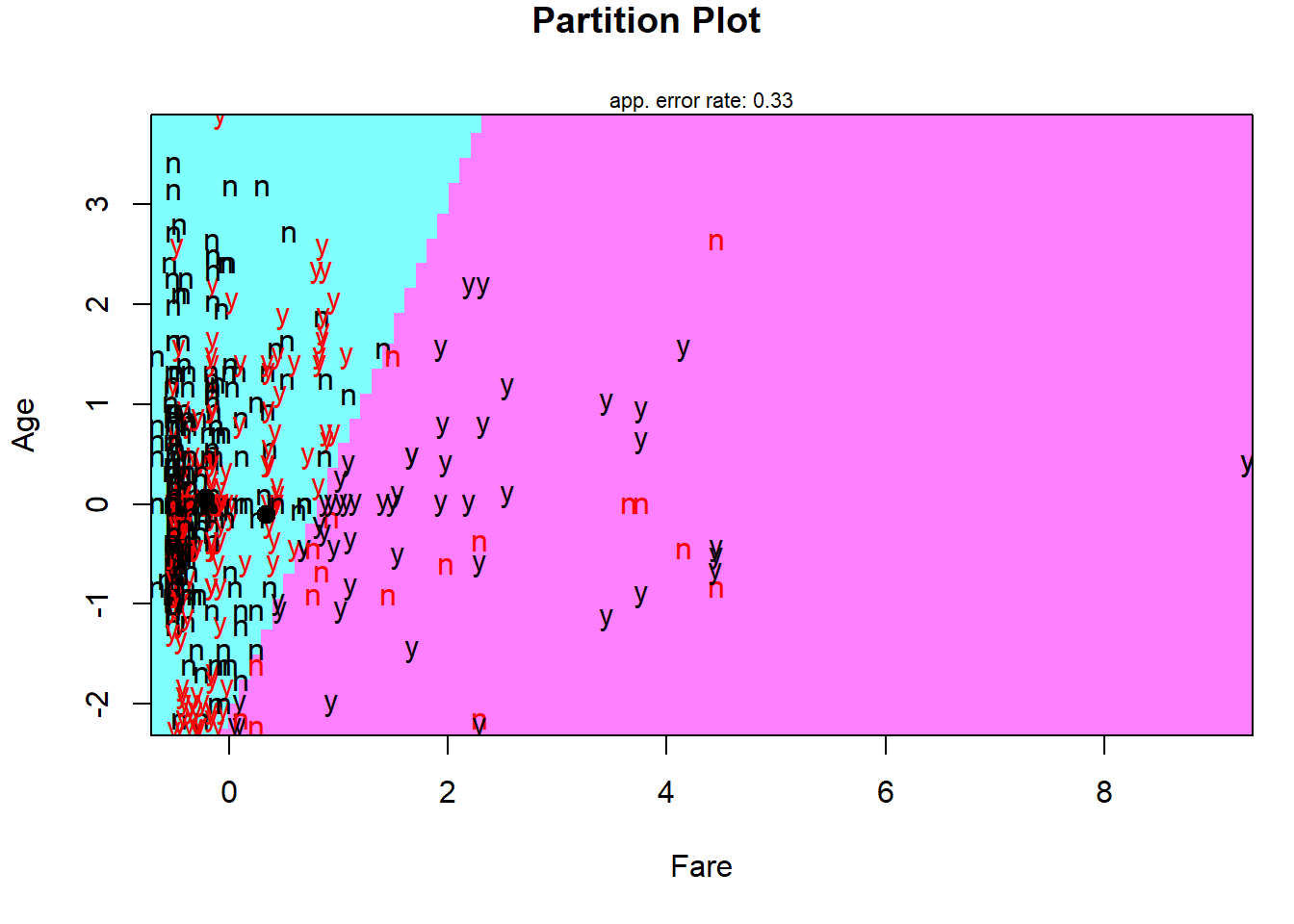

Result! 빨간색은 잘못 분류된 case를 의미하며, 직선형태로 분류 영역이 나뉘어져 있다는 것을 알 수 있다.

7.7.2 모형 평가

Caution! 모형 평가를 위해 Test Dataset에 대한 예측 class/확률이 필요하며, 함수 predict()를 이용하여 생성한다.

# 예측 class와 예측 확률 생성
titanic.lda.pred <- predict(titanic.lda, 
                            newdata = titanic.ted.Imp[,-1])   # Test Dataset including Only 예측 변수   

titanic.lda.pred %>%                                       
  as_tibble

# A tibble: 266 × 3
   class posterior[,"no"] [,"yes"] x[,"LD1"]
   <fct>            <dbl>    <dbl>     <dbl>
 1 no               0.554    0.446    0.464 
 2 no               0.670    0.330   -0.282 
 3 no               0.625    0.375    0.0172
 4 no               0.771    0.229   -1.05  
 5 no               0.624    0.376    0.0239
 6 no               0.683    0.317   -0.373 
 7 no               0.598    0.402    0.192 
 8 no               0.810    0.190   -1.40  
 9 no               0.680    0.320   -0.348 
10 no               0.521    0.479    0.664 
# ℹ 256 more rows

Result! 함수 predict()는 3개의 결과를 리스트로 반환한다.

class : 예측 class
posterior : 각 클래스에 대한 예측 확률(사후 확률)
x : 판별점수

7.7.2.1 ConfusionMatrix

CM   <- caret::confusionMatrix(titanic.lda.pred$class, titanic.ted.Imp$Survived, 
                               positive = "yes")        # confusionMatrix(예측 class, 실제 class, positive = "관심 class")
CM

Confusion Matrix and Statistics

          Reference
Prediction  no yes
       no  159  85
       yes   5  17
                                          
               Accuracy : 0.6617          
                 95% CI : (0.6014, 0.7183)
    No Information Rate : 0.6165          
    P-Value [Acc > NIR] : 0.07266         
                                          
                  Kappa : 0.1599          
                                          
 Mcnemar's Test P-Value : < 2e-16         
                                          
            Sensitivity : 0.16667         
            Specificity : 0.96951         
         Pos Pred Value : 0.77273         
         Neg Pred Value : 0.65164         
             Prevalence : 0.38346         
         Detection Rate : 0.06391         
   Detection Prevalence : 0.08271         
      Balanced Accuracy : 0.56809         
                                          
       'Positive' Class : yes

7.7.2.2 ROC 곡선

ac  <- titanic.ted.Imp$Survived                         # Test Dataset의 실제 class 
pp  <- as.numeric(titanic.lda.pred$posterior[,2])       # "Survived = yes"에 대한 예측 확률을 수치형으로 변환

7.7.2.2.1 Package “pROC”

pacman::p_load("pROC")

lda.roc  <- roc(ac, pp, plot = T, col = "gray")         # roc(실제 class, 예측 확률)
auc      <- round(auc(lda.roc), 3)
legend("bottomright", legend = auc, bty = "n")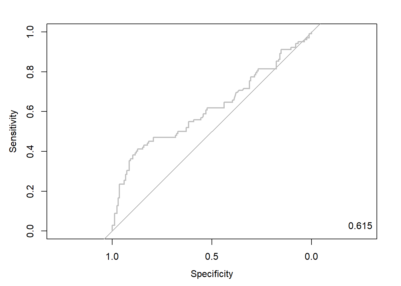

Caution! Package "pROC"를 통해 출력한 ROC 곡선은 다양한 함수를 이용해서 그래프를 수정할 수 있다.

# 함수 plot.roc() 이용
plot.roc(lda.roc,   
         col="gray",                                    # Line Color
         print.auc = TRUE,                              # AUC 출력 여부
         print.auc.col = "red",                         # AUC 글씨 색깔
         print.thres = TRUE,                            # Cutoff Value 출력 여부
         print.thres.pch = 19,                          # Cutoff Value를 표시하는 도형 모양
         print.thres.col = "red",                       # Cutoff Value를 표시하는 도형의 색깔
         auc.polygon = TRUE,                            # 곡선 아래 면적에 대한 여부
         auc.polygon.col = "gray90")                    # 곡선 아래 면적의 색깔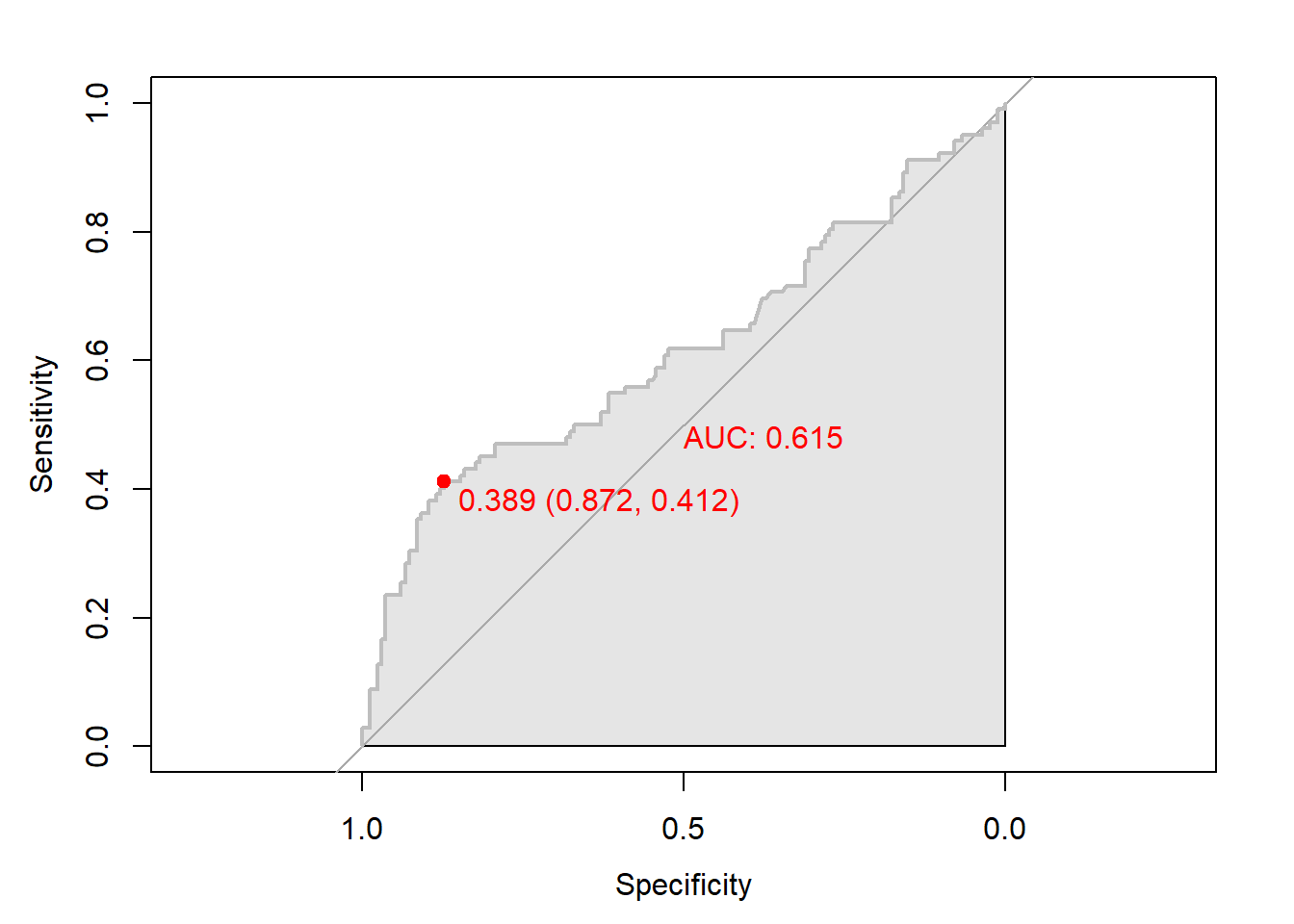

# 함수 ggroc() 이용
ggroc(lda.roc) +
annotate(geom = "text", x = 0.9, y = 1.0,
label = paste("AUC = ", auc),
size = 5,
color="red") +
theme_bw()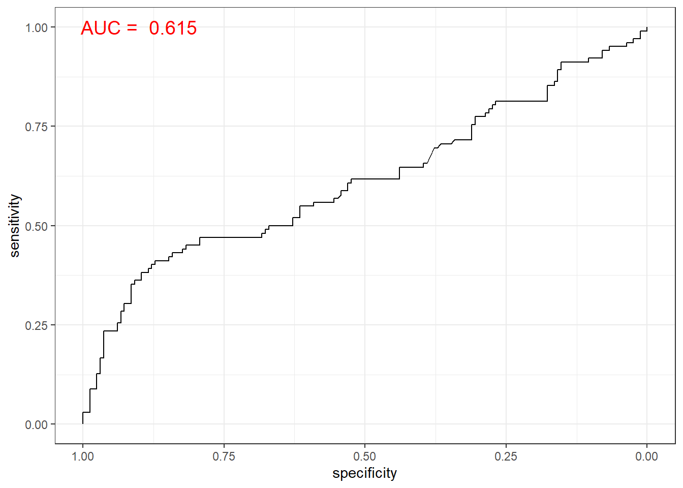

7.7.2.2.2 Package “Epi”

pacman::p_load("Epi")       
# install_version("etm", version = "1.1", repos = "http://cran.us.r-project.org")

ROC(pp, ac, plot = "ROC")                                  # ROC(예측 확률, 실제 class)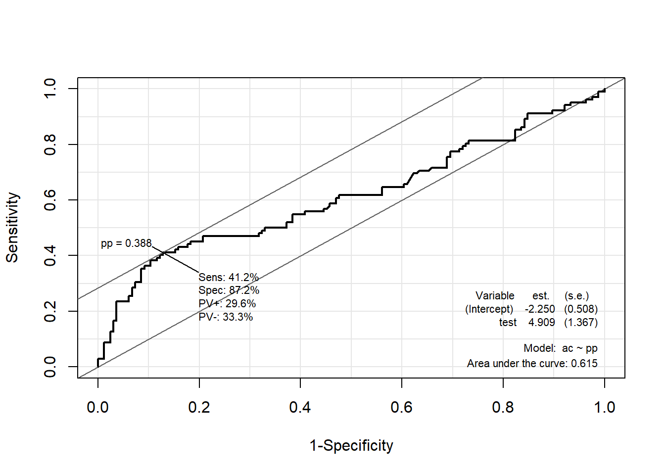

7.7.2.2.3 Package “ROCR”

pacman::p_load("ROCR")

lda.pred <- prediction(pp, ac)                             # prediction(예측 확률, 실제 class)    

lda.perf <- performance(lda.pred, "tpr", "fpr")            # performance(, "민감도", "1-특이도")                      
plot(lda.perf, col = "gray")                               # ROC Curve

perf.auc   <- performance(lda.pred, "auc")                 # AUC
auc        <- attributes(perf.auc)$y.values 
legend("bottomright", legend = auc, bty = "n")

7.7.2.3 향상 차트

7.7.2.3.1 Package “ROCR”

lda.pred <- performance(lda.pred, "lift", "rpp")          # Lift Chart
plot(lda.pred, main = "lift curve", 
     colorize = T,                                        # Coloring according to cutoff
     lwd = 2)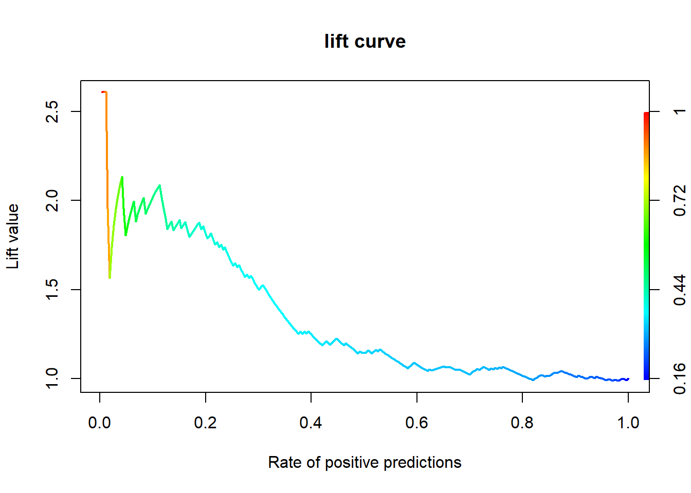

7.7.2.4 오분류표

# 오분류표
lda.ctbl <- table(titanic.ted.Imp$Survived,                # Test Dataset의 실제 class 
                  titanic.lda.pred$class)                  # 예측 class

lda.ctbl

     
       no yes
  no  159   5
  yes  85  17

Desc(lda.ctbl,                                         
     digits = 4)

------------------------------------------------------------------------------------------------------------------------------------------------------------------------------------------------------ 
lda.ctbl (table)

Summary: 
n: 266, rows: 2, columns: 2

Pearson's Chi-squared test (cont. adj):
  X-squared = 13.629, df = 1, p-value = 0.0002227
Fisher's exact test p-value = 0.0001416
McNemar's chi-squared = 69.344, df = 1, p-value < 2.2e-16

                    estimate  lwr.ci  upr.ci'
                                            
odds ratio            6.3600  2.2676 17.8382
rel. risk (col1)      1.1634  1.0623  1.2742
rel. risk (col2)      0.1829  0.0696  0.4806


Contingency Coeff.     0.234
Cramer's V             0.240
Kendall Tau-b          0.240

                                         
                   no       yes       Sum
                                         
no    freq        159         5       164
      perc   59.7744%   1.8797%  61.6541%
      p.row  96.9512%   3.0488%         .
      p.col  65.1639%  22.7273%         .
                                         
yes   freq         85        17       102
      perc   31.9549%   6.3910%  38.3459%
      p.row  83.3333%  16.6667%         .
      p.col  34.8361%  77.2727%         .
                                         
Sum   freq        244        22       266
      perc   91.7293%   8.2707% 100.0000%
      p.row         .         .         .
      p.col         .         .         .
                                         

----------
' 95% conf. level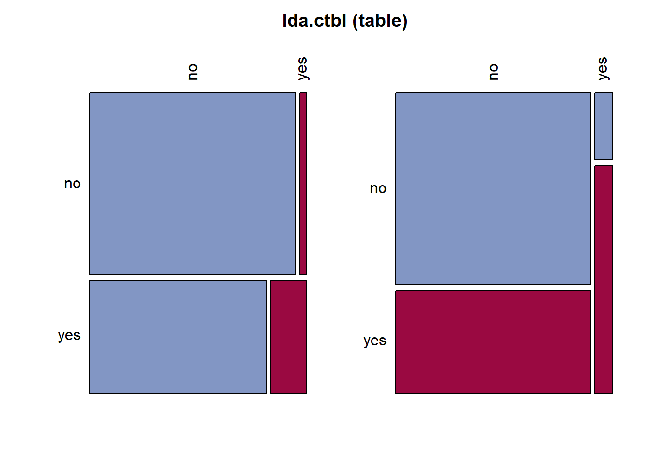

Result! Test Dataset에 대해서 Target “Survived”의 “no”에 속하는 164개의 case 중 159개(159/164=97.0%)는 “no”로 제대로 분류되었으나 5개(5/164=3.0%)는 “yes”로 잘못 분류되었다. 또한, Target “Survived”의 “yes”에 속하는 102개의 case 중 17개(17/102=16.7%)는 “yes”로 제대로 분류되었으나 85개(85/102=83.3%)는 “no”로 잘못 분류되었다. 유도된 선형판별함수에 대한 오분류율은 (5+85)/266=33.8%이며, 정확도는 (159+17)/266=66.2%이다.

7.8 이차판별분석(QDA)

7.8.1 모형 훈련

Caution! Package "MASS"에서 제공하는 함수 qda()를 통해 이차판별함수를 얻을 수 있다.

titanic.qda <- qda(Survived ~ .,     
                   # prior = c(1/2, 1/2),            # 사전확률
                   data = titanic.trd.Imp)      

titanic.qda

Call:
qda(Survived ~ ., data = titanic.trd.Imp)

Prior probabilities of groups:
   no   yes 
0.616 0.384 

Group means:
            Age       Fare      FamSize
no   0.06357863 -0.2127082  0.006151633
yes -0.10199071  0.3412194 -0.009868244

Caution! 이차판별분석에서는 판별계수를 출력하지 않는다.

# 두 예측 변수 "Age"와 "Fare"에 대해 이차판별분석에 기초한 관측값의 분류 결과
partimat(Survived ~ Age + Fare,    
         data = titanic.trd.Imp,
         method = "qda")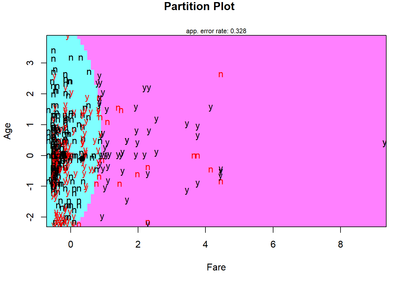

Result! 빨간색은 잘못 분류된 case를 의미한다. 선형판별분석에서 살펴본 그림과 달리 곡선형태로 분류 영역이 나뉘어져 있다는 것을 알 수 있다.

7.8.2 모형 평가

Caution! 모형 평가를 위해 Test Dataset에 대한 예측 class/확률이 필요하며, 함수 predict()를 이용하여 생성한다.

# 예측 class와 예측 확률 생성
titanic.qda.pred <- predict(titanic.qda, 
                            newdata = titanic.ted.Imp[,-1])   # Test Dataset including Only 예측 변수   

titanic.qda.pred %>%                                       
  as_tibble

# A tibble: 266 × 2
   class posterior[,"no"]  [,"yes"]
   <fct>            <dbl>     <dbl>
 1 yes              0.446 0.554    
 2 no               0.569 0.431    
 3 no               0.715 0.285    
 4 no               0.710 0.290    
 5 no               0.981 0.0186   
 6 no               0.751 0.249    
 7 no               0.688 0.312    
 8 no               1.00  0.0000362
 9 no               0.746 0.254    
10 no               0.631 0.369    
# ℹ 256 more rows

7.8.2.1 ConfusionMatrix

CM   <- caret::confusionMatrix(titanic.qda.pred$class, titanic.ted.Imp$Survived, 
                               positive = "yes")        # confusionMatrix(예측 class, 실제 class, positive = "관심 class")
CM

Confusion Matrix and Statistics

          Reference
Prediction  no yes
       no  157  81
       yes   7  21
                                          
               Accuracy : 0.6692          
                 95% CI : (0.6091, 0.7254)
    No Information Rate : 0.6165          
    P-Value [Acc > NIR] : 0.04336         
                                          
                  Kappa : 0.1891          
                                          
 Mcnemar's Test P-Value : 7.149e-15       
                                          
            Sensitivity : 0.20588         
            Specificity : 0.95732         
         Pos Pred Value : 0.75000         
         Neg Pred Value : 0.65966         
             Prevalence : 0.38346         
         Detection Rate : 0.07895         
   Detection Prevalence : 0.10526         
      Balanced Accuracy : 0.58160         
                                          
       'Positive' Class : yes

7.8.2.2 ROC 곡선

ac  <- titanic.ted.Imp$Survived                         # Test Dataset의 실제 class 
pp  <- as.numeric(titanic.qda.pred$posterior[,2])       # "Survived = yes"에 대한 예측 확률을 수치형으로 변환

7.8.2.2.1 Package “pROC”

pacman::p_load("pROC")

qda.roc  <- roc(ac, pp, plot = T, col = "gray")         # roc(실제 class, 예측 확률)
auc      <- round(auc(qda.roc), 3)
legend("bottomright", legend = auc, bty = "n")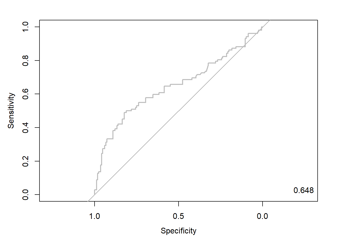

Caution! Package "pROC"를 통해 출력한 ROC 곡선은 다양한 함수를 이용해서 그래프를 수정할 수 있다.

# 함수 plot.roc() 이용
plot.roc(qda.roc,   
         col="gray",                                    # Line Color
         print.auc = TRUE,                              # AUC 출력 여부
         print.auc.col = "red",                         # AUC 글씨 색깔
         print.thres = TRUE,                            # Cutoff Value 출력 여부
         print.thres.pch = 19,                          # Cutoff Value를 표시하는 도형 모양
         print.thres.col = "red",                       # Cutoff Value를 표시하는 도형의 색깔
         auc.polygon = TRUE,                            # 곡선 아래 면적에 대한 여부
         auc.polygon.col = "gray90")                    # 곡선 아래 면적의 색깔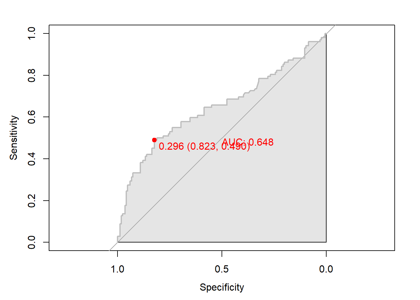

# 함수 ggroc() 이용
ggroc(qda.roc) +
annotate(geom = "text", x = 0.9, y = 1.0,
label = paste("AUC = ", auc),
size = 5,
color="red") +
theme_bw()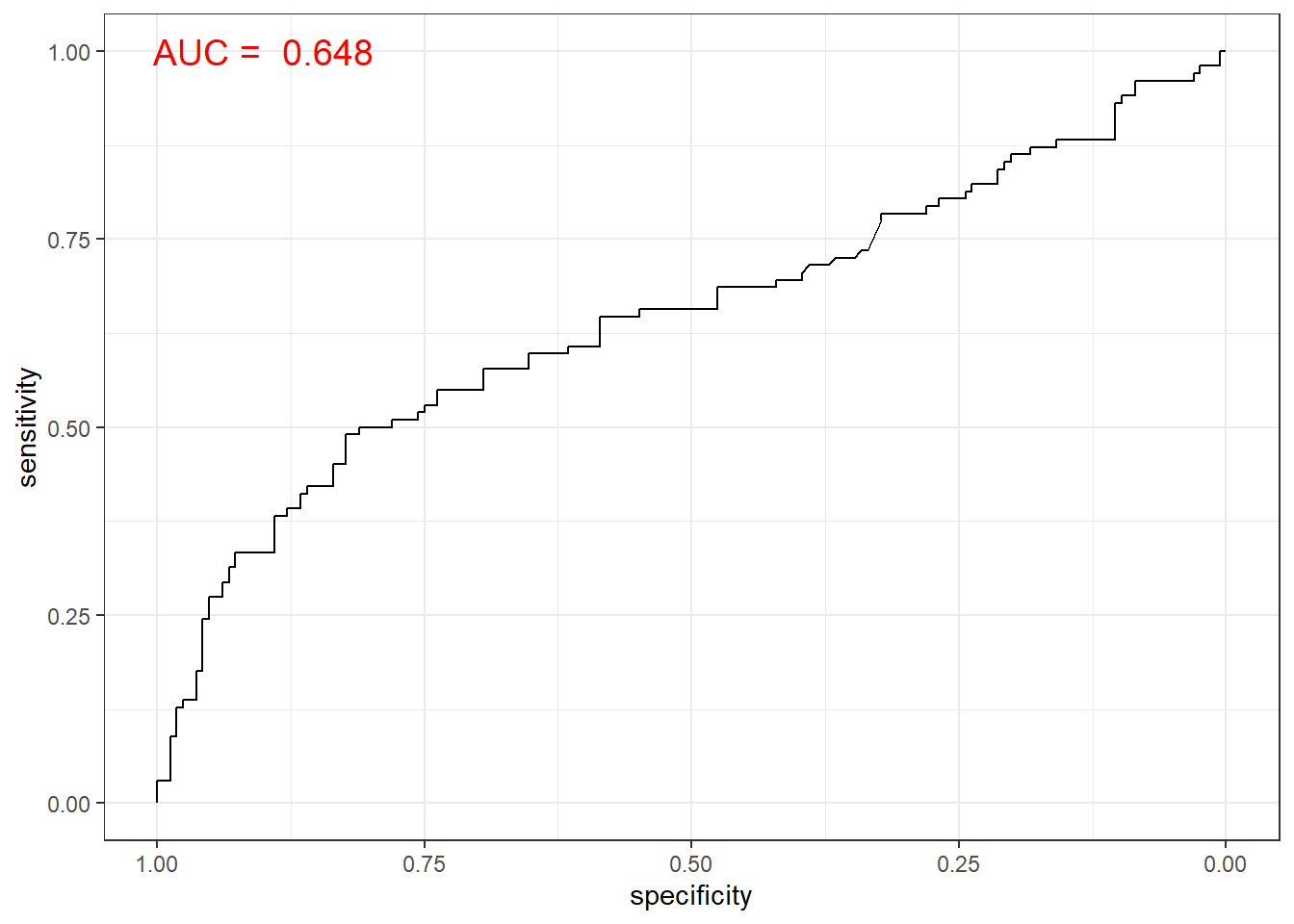

7.8.2.2.2 Package “Epi”

pacman::p_load("Epi")       
# install_version("etm", version = "1.1", repos = "http://cran.us.r-project.org")

ROC(pp, ac, plot = "ROC")                                  # ROC(예측 확률, 실제 class)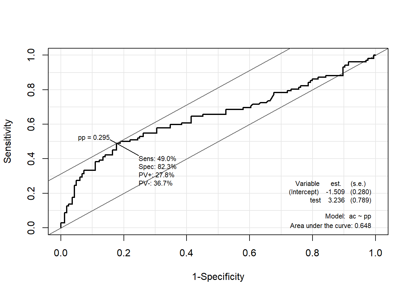

7.8.2.2.3 Package “ROCR”

pacman::p_load("ROCR")

qda.pred <- prediction(pp, ac)                             # prediction(예측 확률, 실제 class)    

qda.perf <- performance(qda.pred, "tpr", "fpr")            # performance(, "민감도", "1-특이도")                      
plot(qda.perf, col = "gray")                               # ROC Curve

perf.auc   <- performance(qda.pred, "auc")                 # AUC
auc        <- attributes(perf.auc)$y.values 
legend("bottomright", legend = auc, bty = "n")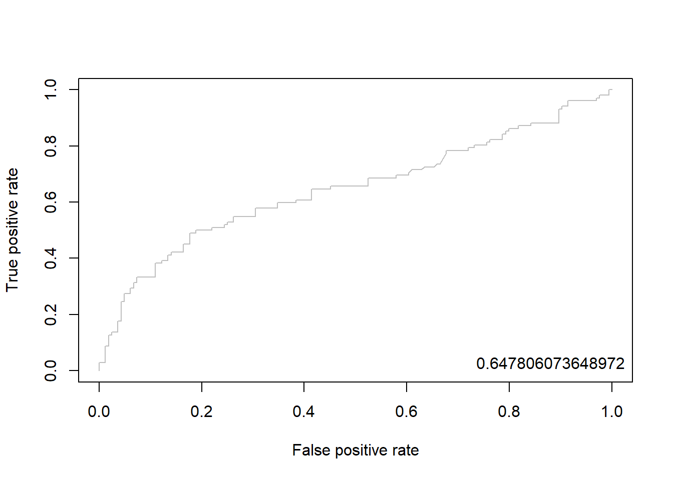

7.8.2.3 향상 차트

7.8.2.3.1 Package “ROCR”

qda.pred <- performance(qda.pred, "lift", "rpp")          # Lift Chart
plot(qda.pred, main = "lift curve", 
     colorize = T,                                        # Coloring according to cutoff
     lwd = 2)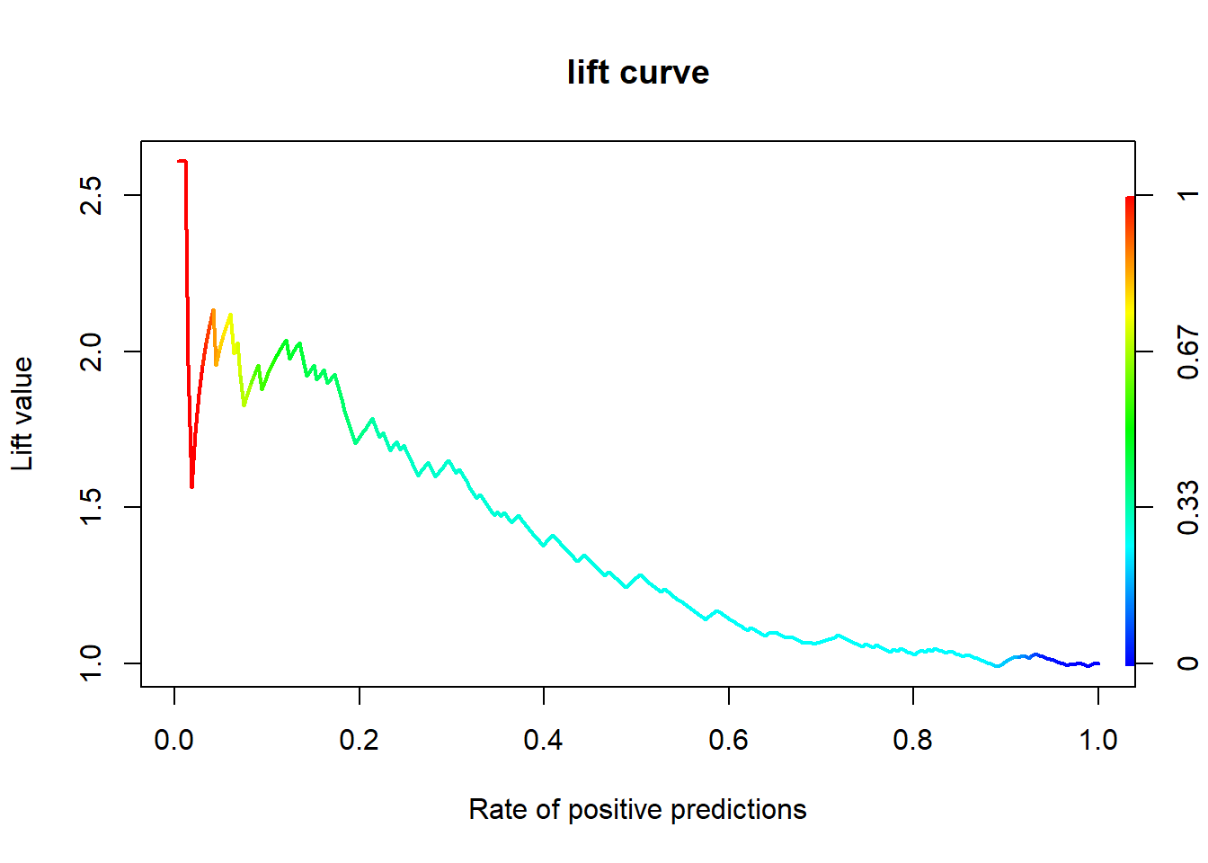

7.8.2.4 오분류표

# 오분류표
qda.ctbl <- table(titanic.ted.Imp$Survived,                # Test Dataset의 실제 class 
                  titanic.qda.pred$class)                  # 예측 class

qda.ctbl

     
       no yes
  no  157   7
  yes  81  21

Desc(qda.ctbl,                                          
     digits = 4)

------------------------------------------------------------------------------------------------------------------------------------------------------------------------------------------------------ 
qda.ctbl (table)

Summary: 
n: 266, rows: 2, columns: 2

Pearson's Chi-squared test (cont. adj):
  X-squared = 16.093, df = 1, p-value = 6.03e-05
Fisher's exact test p-value = 4.7e-05
McNemar's chi-squared = 60.557, df = 1, p-value = 7.149e-15

                    estimate  lwr.ci  upr.ci'
                                            
odds ratio            5.8148  2.3726 14.2513
rel. risk (col1)      1.2055  1.0865  1.3376
rel. risk (col2)      0.2073  0.0914  0.4702


Contingency Coeff.     0.250
Cramer's V             0.259
Kendall Tau-b          0.259

                                         
                   no       yes       Sum
                                         
no    freq        157         7       164
      perc   59.0226%   2.6316%  61.6541%
      p.row  95.7317%   4.2683%         .
      p.col  65.9664%  25.0000%         .
                                         
yes   freq         81        21       102
      perc   30.4511%   7.8947%  38.3459%
      p.row  79.4118%  20.5882%         .
      p.col  34.0336%  75.0000%         .
                                         
Sum   freq        238        28       266
      perc   89.4737%  10.5263% 100.0000%
      p.row         .         .         .
      p.col         .         .         .
                                         

----------
' 95% conf. level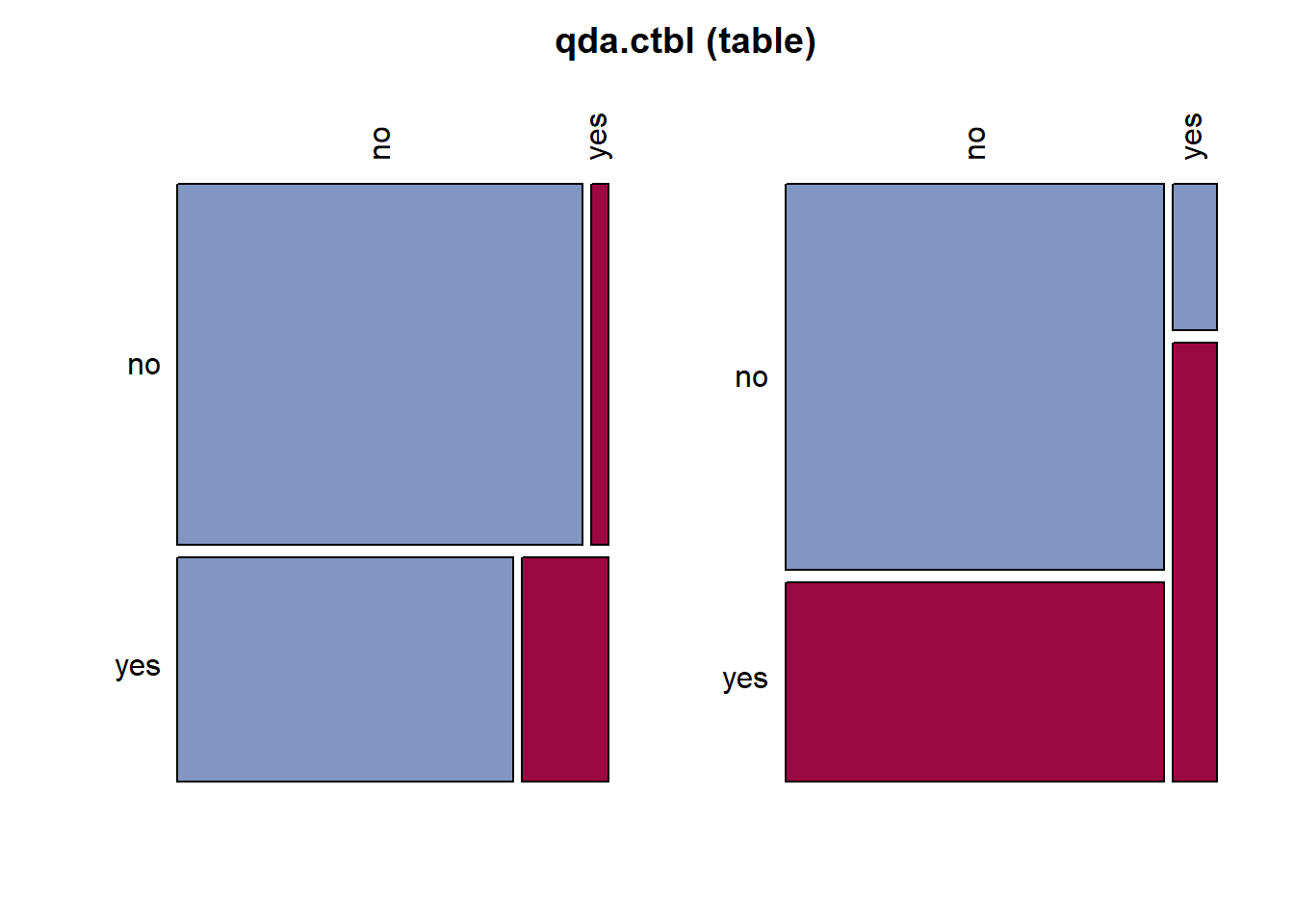

Result! Test Dataset에 대해서 Target “Survived”의 “no”에 속하는 164개의 case 중 157개(157/164=95.7%)는 “no”로 제대로 분류되었으나 7개(7/164=4.3%)는 “yes”로 잘못 분류되었다. 또한, Target “Survived”의 “yes”에 속하는 102개의 case 중 21개(21/102=20.6%)는 “yes”로 제대로 분류되었으나 81개(81/102=79.4%)는 “no”로 잘못 분류되었다. 유도된 이차판별함수에 대한 오분류율은 (7+81)/266=33.1%이며, 정확도는 (157+21)/266=66.9%이다.