pacman::p_load("data.table", "dplyr", "tidyr",
               "caret",
               "ggplot2", "GGally",
               "e1071")

titanic <- fread("../Titanic.csv")                                      # 데이터 불러오기

titanic %>%
as_tibble6 Support Vector Machine with Radial Basis Kernel
Support Vector Machine의 장점
- 분류 경계가 직사각형만 가능한 의사결정나무의 단점을 해결할 수 있다.
- 복잡한 비선형 결정 경계를 학습하는데 유용하다.
- 예측 변수에 분포를 가정하지 않는다.
Support Vector Machine의 단점
- 초모수가 매우 많으며, 초모수에 민감하다.
- 최적의 모형을 찾기 위해 다양한 커널과 초모수의 조합을 평가해야 한다.
- 모형 훈련이 느리다.
- 연속형 예측 변수만 가능하다.
- 범주형 예측 변수는 더미 또는 원-핫 인코딩 변환을 수행해야 한다.
- 해석하기 어려운 복잡한 블랙박스 모형이다.
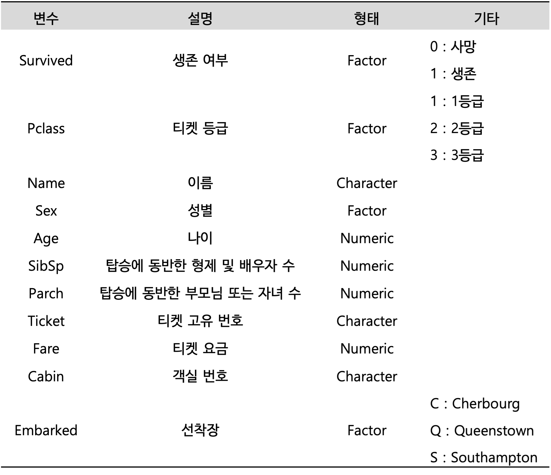
실습 자료 : 1912년 4월 15일 타이타닉호 침몰 당시 탑승객들의 정보를 기록한 데이터셋이며, 총 11개의 변수를 포함하고 있다. 이 자료에서 Target은
Survived이다.
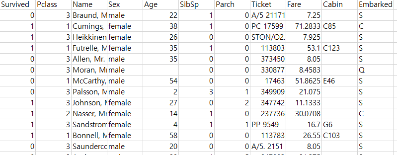
6.1 데이터 불러오기
# A tibble: 891 × 11
   Survived Pclass Name                                                Sex      Age SibSp Parch Ticket            Fare Cabin  Embarked
      <int>  <int> <chr>                                               <chr>  <dbl> <int> <int> <chr>            <dbl> <chr>  <chr>
 1        0      3 Braund, Mr. Owen Harris                             male      22     1     0 A/5 21171         7.25 ""     S
 2        1      1 Cumings, Mrs. John Bradley (Florence Briggs Thayer) female    38     1     0 PC 17599         71.3  "C85"  C
 3        1      3 Heikkinen, Miss. Laina                              female    26     0     0 STON/O2. 3101282  7.92 ""     S
 4        1      1 Futrelle, Mrs. Jacques Heath (Lily May Peel)        female    35     1     0 113803           53.1  "C123" S
 5        0      3 Allen, Mr. William Henry                            male      35     0     0 373450            8.05 ""     S
 6        0      3 Moran, Mr. James                                    male      NA     0     0 330877            8.46 ""     Q
 7        0      1 McCarthy, Mr. Timothy J                             male      54     0     0 17463            51.9  "E46"  S
 8        0      3 Palsson, Master. Gosta Leonard                      male       2     3     1 349909           21.1  ""     S
 9        1      3 Johnson, Mrs. Oscar W (Elisabeth Vilhelmina Berg)   female    27     0     2 347742           11.1  ""     S
10        1      2 Nasser, Mrs. Nicholas (Adele Achem)                 female    14     1     0 237736           30.1  ""     C
# ℹ 881 more rows
6.2 데이터 전처리 I
titanic %<>%
  data.frame() %>%                                                      # Data Frame 형태로 변환
  mutate(Survived = ifelse(Survived == 1, "yes", "no"))                 # Target을 문자형 변수로 변환

# 1. Convert to Factor
fac.col <- c("Pclass", "Sex",
             # Target
             "Survived")

titanic <- titanic %>%
  mutate_at(fac.col, as.factor)                                         # 범주형으로 변환

glimpse(titanic)                                                        # 데이터 구조 확인
Rows: 891
Columns: 11
$ Survived <fct> no, yes, yes, yes, no, no, no, no, yes, yes, yes, yes, no, no, no, yes, no, yes, no, yes, no, yes, yes, yes, no, yes, no, no, yes, no, no, yes, yes, no, no, no, yes, no, no, yes, no…
$ Pclass <fct> 3, 1, 3, 1, 3, 3, 1, 3, 3, 2, 3, 1, 3, 3, 3, 2, 3, 2, 3, 3, 2, 2, 3, 1, 3, 3, 3, 1, 3, 3, 1, 1, 3, 2, 1, 1, 3, 3, 3, 3, 3, 2, 3, 2, 3, 3, 3, 3, 3, 3, 3, 3, 1, 2, 1, 1, 2, 3, 2, 3, 3…
$ Name <chr> "Braund, Mr. Owen Harris", "Cumings, Mrs. John Bradley (Florence Briggs Thayer)", "Heikkinen, Miss. Laina", "Futrelle, Mrs. Jacques Heath (Lily May Peel)", "Allen, Mr. William Henry…
$ Sex <fct> male, female, female, female, male, male, male, male, female, female, female, female, male, male, female, female, male, male, female, female, male, male, female, male, female, femal…
$ Age <dbl> 22.0, 38.0, 26.0, 35.0, 35.0, NA, 54.0, 2.0, 27.0, 14.0, 4.0, 58.0, 20.0, 39.0, 14.0, 55.0, 2.0, NA, 31.0, NA, 35.0, 34.0, 15.0, 28.0, 8.0, 38.0, NA, 19.0, NA, NA, 40.0, NA, NA, 66.…
$ SibSp <int> 1, 1, 0, 1, 0, 0, 0, 3, 0, 1, 1, 0, 0, 1, 0, 0, 4, 0, 1, 0, 0, 0, 0, 0, 3, 1, 0, 3, 0, 0, 0, 1, 0, 0, 1, 1, 0, 0, 2, 1, 1, 1, 0, 1, 0, 0, 1, 0, 2, 1, 4, 0, 1, 1, 0, 0, 0, 0, 1, 5, 0…
$ Parch <int> 0, 0, 0, 0, 0, 0, 0, 1, 2, 0, 1, 0, 0, 5, 0, 0, 1, 0, 0, 0, 0, 0, 0, 0, 1, 5, 0, 2, 0, 0, 0, 0, 0, 0, 0, 0, 0, 0, 0, 0, 0, 0, 0, 2, 0, 0, 0, 0, 0, 0, 1, 0, 0, 0, 1, 0, 0, 0, 2, 2, 0…
$ Ticket <chr> "A/5 21171", "PC 17599", "STON/O2. 3101282", "113803", "373450", "330877", "17463", "349909", "347742", "237736", "PP 9549", "113783", "A/5. 2151", "347082", "350406", "248706", "38…
$ Fare <dbl> 7.2500, 71.2833, 7.9250, 53.1000, 8.0500, 8.4583, 51.8625, 21.0750, 11.1333, 30.0708, 16.7000, 26.5500, 8.0500, 31.2750, 7.8542, 16.0000, 29.1250, 13.0000, 18.0000, 7.2250, 26.0000,…
$ Cabin <chr> "", "C85", "", "C123", "", "", "E46", "", "", "", "G6", "C103", "", "", "", "", "", "", "", "", "", "D56", "", "A6", "", "", "", "C23 C25 C27", "", "", "", "B78", "", "", "", "", ""…
$ Embarked <chr> "S", "C", "S", "S", "S", "Q", "S", "S", "S", "C", "S", "S", "S", "S", "S", "S", "Q", "S", "S", "C", "S", "S", "Q", "S", "S", "S", "C", "S", "Q", "S", "C", "C", "Q", "S", "C", "S", "…# 2. Generate New Variable
titanic <- titanic %>%
mutate(FamSize = SibSp + Parch) # "FamSize = 형제 및 배우자 수 + 부모님 및 자녀 수"로 가족 수를 의미하는 새로운 변수
glimpse(titanic) # 데이터 구조 확인Rows: 891
Columns: 12
$ Survived <fct> no, yes, yes, yes, no, no, no, no, yes, yes, yes, yes, no, no, no, yes, no, yes, no, yes, no, yes, yes, yes, no, yes, no, no, yes, no, no, yes, yes, no, no, no, yes, no, no, yes, no…
$ Pclass <fct> 3, 1, 3, 1, 3, 3, 1, 3, 3, 2, 3, 1, 3, 3, 3, 2, 3, 2, 3, 3, 2, 2, 3, 1, 3, 3, 3, 1, 3, 3, 1, 1, 3, 2, 1, 1, 3, 3, 3, 3, 3, 2, 3, 2, 3, 3, 3, 3, 3, 3, 3, 3, 1, 2, 1, 1, 2, 3, 2, 3, 3…
$ Name <chr> "Braund, Mr. Owen Harris", "Cumings, Mrs. John Bradley (Florence Briggs Thayer)", "Heikkinen, Miss. Laina", "Futrelle, Mrs. Jacques Heath (Lily May Peel)", "Allen, Mr. William Henry…
$ Sex <fct> male, female, female, female, male, male, male, male, female, female, female, female, male, male, female, female, male, male, female, female, male, male, female, male, female, femal…
$ Age <dbl> 22.0, 38.0, 26.0, 35.0, 35.0, NA, 54.0, 2.0, 27.0, 14.0, 4.0, 58.0, 20.0, 39.0, 14.0, 55.0, 2.0, NA, 31.0, NA, 35.0, 34.0, 15.0, 28.0, 8.0, 38.0, NA, 19.0, NA, NA, 40.0, NA, NA, 66.…
$ SibSp <int> 1, 1, 0, 1, 0, 0, 0, 3, 0, 1, 1, 0, 0, 1, 0, 0, 4, 0, 1, 0, 0, 0, 0, 0, 3, 1, 0, 3, 0, 0, 0, 1, 0, 0, 1, 1, 0, 0, 2, 1, 1, 1, 0, 1, 0, 0, 1, 0, 2, 1, 4, 0, 1, 1, 0, 0, 0, 0, 1, 5, 0…
$ Parch <int> 0, 0, 0, 0, 0, 0, 0, 1, 2, 0, 1, 0, 0, 5, 0, 0, 1, 0, 0, 0, 0, 0, 0, 0, 1, 5, 0, 2, 0, 0, 0, 0, 0, 0, 0, 0, 0, 0, 0, 0, 0, 0, 0, 2, 0, 0, 0, 0, 0, 0, 1, 0, 0, 0, 1, 0, 0, 0, 2, 2, 0…
$ Ticket <chr> "A/5 21171", "PC 17599", "STON/O2. 3101282", "113803", "373450", "330877", "17463", "349909", "347742", "237736", "PP 9549", "113783", "A/5. 2151", "347082", "350406", "248706", "38…
$ Fare <dbl> 7.2500, 71.2833, 7.9250, 53.1000, 8.0500, 8.4583, 51.8625, 21.0750, 11.1333, 30.0708, 16.7000, 26.5500, 8.0500, 31.2750, 7.8542, 16.0000, 29.1250, 13.0000, 18.0000, 7.2250, 26.0000,…
$ Cabin <chr> "", "C85", "", "C123", "", "", "E46", "", "", "", "G6", "C103", "", "", "", "", "", "", "", "", "", "D56", "", "A6", "", "", "", "C23 C25 C27", "", "", "", "B78", "", "", "", "", ""…
$ Embarked <chr> "S", "C", "S", "S", "S", "Q", "S", "S", "S", "C", "S", "S", "S", "S", "S", "S", "Q", "S", "S", "C", "S", "S", "Q", "S", "S", "S", "C", "S", "Q", "S", "C", "C", "Q", "S", "C", "S", "…
$ FamSize <int> 1, 1, 0, 1, 0, 0, 0, 4, 2, 1, 2, 0, 0, 6, 0, 0, 5, 0, 1, 0, 0, 0, 0, 0, 4, 6, 0, 5, 0, 0, 0, 1, 0, 0, 1, 1, 0, 0, 2, 1, 1, 1, 0, 3, 0, 0, 1, 0, 2, 1, 5, 0, 1, 1, 1, 0, 0, 0, 3, 7, 0…# 3. Select Variables used for Analysis
titanic1 <- titanic %>%
select(Survived, Pclass, Sex, Age, Fare, FamSize) # 분석에 사용할 변수 선택
# 4. Convert One-hot Encoding for 범주형 예측 변수
dummies <- dummyVars(formula = ~ ., # formula : ~ 예측 변수 / "." : data에 포함된 모든 변수를 의미
data = titanic1[,-1], # Dataset including Only 예측 변수 -> Target 제외
fullRank = FALSE) # fullRank = TRUE : Dummy Variable, fullRank = FALSE : One-hot Encoding
titanic.Var <- predict(dummies, newdata = titanic1) %>% # 범주형 예측 변수에 대한 One-hot Encoding 변환
data.frame() # Data Frame 형태로 변환
glimpse(titanic.Var) # 데이터 구조 확인Rows: 891
Columns: 8
$ Pclass.1 <dbl> 0, 1, 0, 1, 0, 0, 1, 0, 0, 0, 0, 1, 0, 0, 0, 0, 0, 0, 0, 0, 0, 0, 0, 1, 0, 0, 0, 1, 0, 0, 1, 1, 0, 0, 1, 1, 0, 0, 0, 0, 0, 0, 0, 0, 0, 0, 0, 0, 0, 0, 0, 0, 1, 0, 1, 1, 0, 0, 0, 0,…
$ Pclass.2 <dbl> 0, 0, 0, 0, 0, 0, 0, 0, 0, 1, 0, 0, 0, 0, 0, 1, 0, 1, 0, 0, 1, 1, 0, 0, 0, 0, 0, 0, 0, 0, 0, 0, 0, 1, 0, 0, 0, 0, 0, 0, 0, 1, 0, 1, 0, 0, 0, 0, 0, 0, 0, 0, 0, 1, 0, 0, 1, 0, 1, 0,…
$ Pclass.3 <dbl> 1, 0, 1, 0, 1, 1, 0, 1, 1, 0, 1, 0, 1, 1, 1, 0, 1, 0, 1, 1, 0, 0, 1, 0, 1, 1, 1, 0, 1, 1, 0, 0, 1, 0, 0, 0, 1, 1, 1, 1, 1, 0, 1, 0, 1, 1, 1, 1, 1, 1, 1, 1, 0, 0, 0, 0, 0, 1, 0, 1,…
$ Sex.female <dbl> 0, 1, 1, 1, 0, 0, 0, 0, 1, 1, 1, 1, 0, 0, 1, 1, 0, 0, 1, 1, 0, 0, 1, 0, 1, 1, 0, 0, 1, 0, 0, 1, 1, 0, 0, 0, 0, 0, 1, 1, 1, 1, 0, 1, 1, 0, 0, 1, 0, 1, 0, 0, 1, 1, 0, 0, 1, 0, 1, 0,…
$ Sex.male <dbl> 1, 0, 0, 0, 1, 1, 1, 1, 0, 0, 0, 0, 1, 1, 0, 0, 1, 1, 0, 0, 1, 1, 0, 1, 0, 0, 1, 1, 0, 1, 1, 0, 0, 1, 1, 1, 1, 1, 0, 0, 0, 0, 1, 0, 0, 1, 1, 0, 1, 0, 1, 1, 0, 0, 1, 1, 0, 1, 0, 1,…
$ Age <dbl> 22.0, 38.0, 26.0, 35.0, 35.0, NA, 54.0, 2.0, 27.0, 14.0, 4.0, 58.0, 20.0, 39.0, 14.0, 55.0, 2.0, NA, 31.0, NA, 35.0, 34.0, 15.0, 28.0, 8.0, 38.0, NA, 19.0, NA, NA, 40.0, NA, NA, 6…
$ Fare <dbl> 7.2500, 71.2833, 7.9250, 53.1000, 8.0500, 8.4583, 51.8625, 21.0750, 11.1333, 30.0708, 16.7000, 26.5500, 8.0500, 31.2750, 7.8542, 16.0000, 29.1250, 13.0000, 18.0000, 7.2250, 26.000…
$ FamSize <dbl> 1, 1, 0, 1, 0, 0, 0, 4, 2, 1, 2, 0, 0, 6, 0, 0, 5, 0, 1, 0, 0, 0, 0, 0, 4, 6, 0, 5, 0, 0, 0, 1, 0, 0, 1, 1, 0, 0, 2, 1, 1, 1, 0, 3, 0, 0, 1, 0, 2, 1, 5, 0, 1, 1, 1, 0, 0, 0, 3, 7,…# Combine Target with 변환된 예측 변수
titanic.df <- data.frame(Survived = titanic1$Survived,
titanic.Var)
titanic.df %>%
as_tibble# A tibble: 891 × 9
Survived Pclass.1 Pclass.2 Pclass.3 Sex.female Sex.male Age Fare FamSize
<fct> <dbl> <dbl> <dbl> <dbl> <dbl> <dbl> <dbl> <dbl>
1 no 0 0 1 0 1 22 7.25 1
2 yes 1 0 0 1 0 38 71.3 1
3 yes 0 0 1 1 0 26 7.92 0
4 yes 1 0 0 1 0 35 53.1 1
5 no 0 0 1 0 1 35 8.05 0
6 no 0 0 1 0 1 NA 8.46 0
7 no 1 0 0 0 1 54 51.9 0
8 no 0 0 1 0 1 2 21.1 4
9 yes 0 0 1 1 0 27 11.1 2
10 yes 0 1 0 1 0 14 30.1 1
# ℹ 881 more rowsglimpse(titanic.df) # 데이터 구조 확인Rows: 891
Columns: 9
$ Survived <fct> no, yes, yes, yes, no, no, no, no, yes, yes, yes, yes, no, no, no, yes, no, yes, no, yes, no, yes, yes, yes, no, yes, no, no, yes, no, no, yes, yes, no, no, no, yes, no, no, yes, …
$ Pclass.1 <dbl> 0, 1, 0, 1, 0, 0, 1, 0, 0, 0, 0, 1, 0, 0, 0, 0, 0, 0, 0, 0, 0, 0, 0, 1, 0, 0, 0, 1, 0, 0, 1, 1, 0, 0, 1, 1, 0, 0, 0, 0, 0, 0, 0, 0, 0, 0, 0, 0, 0, 0, 0, 0, 1, 0, 1, 1, 0, 0, 0, 0,…
$ Pclass.2 <dbl> 0, 0, 0, 0, 0, 0, 0, 0, 0, 1, 0, 0, 0, 0, 0, 1, 0, 1, 0, 0, 1, 1, 0, 0, 0, 0, 0, 0, 0, 0, 0, 0, 0, 1, 0, 0, 0, 0, 0, 0, 0, 1, 0, 1, 0, 0, 0, 0, 0, 0, 0, 0, 0, 1, 0, 0, 1, 0, 1, 0,…
$ Pclass.3 <dbl> 1, 0, 1, 0, 1, 1, 0, 1, 1, 0, 1, 0, 1, 1, 1, 0, 1, 0, 1, 1, 0, 0, 1, 0, 1, 1, 1, 0, 1, 1, 0, 0, 1, 0, 0, 0, 1, 1, 1, 1, 1, 0, 1, 0, 1, 1, 1, 1, 1, 1, 1, 1, 0, 0, 0, 0, 0, 1, 0, 1,…
$ Sex.female <dbl> 0, 1, 1, 1, 0, 0, 0, 0, 1, 1, 1, 1, 0, 0, 1, 1, 0, 0, 1, 1, 0, 0, 1, 0, 1, 1, 0, 0, 1, 0, 0, 1, 1, 0, 0, 0, 0, 0, 1, 1, 1, 1, 0, 1, 1, 0, 0, 1, 0, 1, 0, 0, 1, 1, 0, 0, 1, 0, 1, 0,…
$ Sex.male <dbl> 1, 0, 0, 0, 1, 1, 1, 1, 0, 0, 0, 0, 1, 1, 0, 0, 1, 1, 0, 0, 1, 1, 0, 1, 0, 0, 1, 1, 0, 1, 1, 0, 0, 1, 1, 1, 1, 1, 0, 0, 0, 0, 1, 0, 0, 1, 1, 0, 1, 0, 1, 1, 0, 0, 1, 1, 0, 1, 0, 1,…
$ Age <dbl> 22.0, 38.0, 26.0, 35.0, 35.0, NA, 54.0, 2.0, 27.0, 14.0, 4.0, 58.0, 20.0, 39.0, 14.0, 55.0, 2.0, NA, 31.0, NA, 35.0, 34.0, 15.0, 28.0, 8.0, 38.0, NA, 19.0, NA, NA, 40.0, NA, NA, 6…
$ Fare <dbl> 7.2500, 71.2833, 7.9250, 53.1000, 8.0500, 8.4583, 51.8625, 21.0750, 11.1333, 30.0708, 16.7000, 26.5500, 8.0500, 31.2750, 7.8542, 16.0000, 29.1250, 13.0000, 18.0000, 7.2250, 26.000…
$ FamSize <dbl> 1, 1, 0, 1, 0, 0, 0, 4, 2, 1, 2, 0, 0, 6, 0, 0, 5, 0, 1, 0, 0, 0, 0, 0, 4, 6, 0, 5, 0, 0, 0, 1, 0, 0, 1, 1, 0, 0, 2, 1, 1, 1, 0, 3, 0, 0, 1, 0, 2, 1, 5, 0, 1, 1, 1, 0, 0, 0, 3, 7,…6.3 데이터 탐색
ggpairs(titanic.df,
        aes(colour = Survived)) +                         # Target의 범주에 따라 색깔을 다르게 표현
  theme_bw()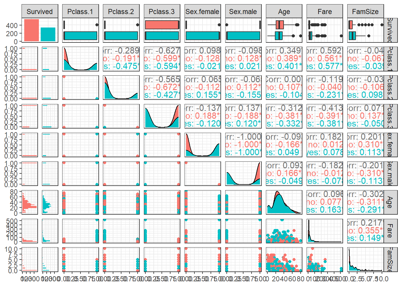
ggpairs(titanic.df,
        aes(colour = Survived, alpha = 0.8)) +            # Target의 범주에 따라 색깔을 다르게 표현
  scale_colour_manual(values = c("purple", "cyan4")) +    # 특정 색깔 지정
  scale_fill_manual(values = c("purple", "cyan4")) +      # 특정 색깔 지정
  theme_bw()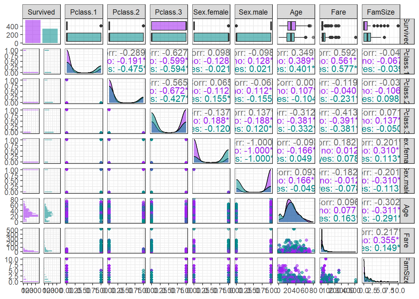
6.4 데이터 분할
# Partition (Training Dataset : Test Dataset = 7:3)
y      <- titanic.df$Survived                           # Target

set.seed(200)
ind    <- createDataPartition(y, p = 0.7, list  =T)     # Index를 이용하여 7:3으로 분할
titanic.trd <- titanic.df[ind$Resample1,]               # Training Dataset
titanic.ted <- titanic.df[-ind$Resample1,]              # Test Dataset
6.5 데이터 전처리 II
# 1. Imputation
titanic.trd.Imp <- titanic.trd %>%
  mutate(Age = replace_na(Age, mean(Age, na.rm = TRUE)))                 # 평균으로 결측값 대체

titanic.ted.Imp <- titanic.ted %>%
  mutate(Age = replace_na(Age, mean(titanic.trd$Age, na.rm = TRUE)))     # Training Dataset을 이용하여 결측값 대체

# 2. Standardization
preProcValues <- preProcess(titanic.trd.Imp,
                            method = c("center", "scale"))               # Standardization 정의 -> Training Dataset에 대한 평균과 표준편차 계산

titanic.trd.Imp <- predict(preProcValues, titanic.trd.Imp)               # Standardization for Training Dataset
titanic.ted.Imp <- predict(preProcValues, titanic.ted.Imp)               # Standardization for Test Dataset

glimpse(titanic.trd.Imp)                                                 # 데이터 구조 확인
Rows: 625
Columns: 9
$ Survived <fct> no, yes, yes, no, no, no, yes, yes, yes, yes, no, no, yes, no, yes, no, yes, no, no, no, yes, no, no, yes, yes, no, no, no, no, no, yes, no, no, no, yes, no, yes, no, no, no, yes,…
$ Pclass.1 <dbl> -0.593506, -0.593506, 1.682207, -0.593506, -0.593506, -0.593506, -0.593506, -0.593506, -0.593506, 1.682207, -0.593506, -0.593506, -0.593506, -0.593506, -0.593506, -0.593506, 1.682…
$ Pclass.2 <dbl> -0.4694145, -0.4694145, -0.4694145, -0.4694145, -0.4694145, -0.4694145, -0.4694145, 2.1269048, -0.4694145, -0.4694145, -0.4694145, -0.4694145, 2.1269048, -0.4694145, -0.4694145, 2…
$ Pclass.3 <dbl> 0.888575, 0.888575, -1.123597, 0.888575, 0.888575, 0.888575, 0.888575, -1.123597, 0.888575, -1.123597, 0.888575, 0.888575, -1.123597, 0.888575, 0.888575, -1.123597, -1.123597, 0.8…
$ Sex.female <dbl> -0.7572241, 1.3184999, 1.3184999, -0.7572241, -0.7572241, -0.7572241, 1.3184999, 1.3184999, 1.3184999, 1.3184999, -0.7572241, 1.3184999, -0.7572241, 1.3184999, 1.3184999, -0.75722…
$ Sex.male <dbl> 0.7572241, -1.3184999, -1.3184999, 0.7572241, 0.7572241, 0.7572241, -1.3184999, -1.3184999, -1.3184999, -1.3184999, 0.7572241, -1.3184999, 0.7572241, -1.3184999, -1.3184999, 0.757…
$ Age <dbl> -0.61306970, -0.30411628, 0.39102893, 0.39102893, 0.00000000, -2.15783684, -0.22687792, -1.23097656, -2.00336012, 2.16751113, 0.69998236, -1.23097656, 0.00000000, 0.08207551, 0.00…
$ Fare <dbl> -0.51776394, -0.50463325, 0.37414970, -0.50220165, -0.49425904, -0.24882814, -0.44222264, -0.07383411, -0.33393441, -0.14232374, -0.05040897, -0.50601052, -0.40590999, -0.30864569…
$ FamSize <dbl> 0.04506631, -0.55421976, 0.04506631, -0.55421976, -0.55421976, 1.84292454, 0.64435239, 0.04506631, 0.64435239, -0.55421976, 3.04149669, -0.55421976, -0.55421976, 0.04506631, -0.55…glimpse(titanic.ted.Imp) # 데이터 구조 확인Rows: 266
Columns: 9
$ Survived <fct> yes, no, no, yes, no, yes, yes, yes, yes, yes, no, no, yes, yes, no, yes, no, yes, yes, no, yes, no, no, no, no, no, no, yes, yes, no, no, no, no, no, no, no, no, no, no, yes, no,…
$ Pclass.1 <dbl> 1.682207, 1.682207, -0.593506, -0.593506, -0.593506, -0.593506, -0.593506, -0.593506, -0.593506, -0.593506, -0.593506, -0.593506, -0.593506, -0.593506, -0.593506, -0.593506, 1.682…
$ Pclass.2 <dbl> -0.4694145, -0.4694145, -0.4694145, 2.1269048, -0.4694145, 2.1269048, -0.4694145, -0.4694145, -0.4694145, 2.1269048, -0.4694145, -0.4694145, 2.1269048, 2.1269048, -0.4694145, 2.12…
$ Pclass.3 <dbl> -1.123597, -1.123597, 0.888575, -1.123597, 0.888575, -1.123597, 0.888575, 0.888575, 0.888575, -1.123597, 0.888575, 0.888575, -1.123597, -1.123597, 0.888575, -1.123597, -1.123597, …
$ Sex.female <dbl> 1.3184999, -0.7572241, -0.7572241, 1.3184999, -0.7572241, -0.7572241, 1.3184999, 1.3184999, -0.7572241, 1.3184999, -0.7572241, -0.7572241, 1.3184999, 1.3184999, -0.7572241, 1.3184…
$ Sex.male <dbl> -1.3184999, 0.7572241, 0.7572241, -1.3184999, 0.7572241, 0.7572241, -1.3184999, -1.3184999, 0.7572241, -1.3184999, 0.7572241, 0.7572241, -1.3184999, -1.3184999, 0.7572241, -1.3184…
$ Age <dbl> 0.62274400, 1.85855771, -0.76754642, 1.93579607, -2.15783684, 0.31379058, -1.15373820, 0.62274400, 0.00000000, -2.08059848, 0.00000000, -0.69030806, -0.07240121, -0.69030806, -0.1…
$ Fare <dbl> 0.727866891, 0.350076786, -0.502201647, -0.347551409, -0.092232621, -0.405909990, -0.502606266, -0.048220525, -0.518168555, 0.150037190, -0.502201647, -0.507064862, -0.153022808, …
$ FamSize <dbl> 0.04506631, -0.55421976, -0.55421976, -0.55421976, 2.44221062, -0.55421976, -0.55421976, 3.04149669, -0.55421976, 1.24363847, -0.55421976, -0.55421976, 0.04506631, -0.55421976, -0…6.6 모형 훈련
Package "e1071"는 Support Vector Machine을 효율적으로 구현할 수 있는 “libsvm”을 R에서 사용할 수 있도록 만든 Package이며, 함수 svm()을 이용하여 Support Vector Machine을 수행할 수 있다. 함수에서 사용할 수 있는 자세한 옵션은 여기를 참고한다.
svm(formula, data, kernel, cost, gamma, probability, ...)formula: Target과 예측 변수의 관계를 표현하기 위한 함수로써 일반적으로Target ~ 예측 변수의 형태로 표현한다.data:formula에 포함하고 있는 변수들의 데이터셋(Data Frame)kernel: Kernel 함수"linear": \(k(\boldsymbol{x}, \boldsymbol{x}') = \boldsymbol{x}\boldsymbol{x}'\)"polynomial": \(k(\boldsymbol{x}, \boldsymbol{x}') = (\gamma \boldsymbol{x}\boldsymbol{x}' + \text{coef0})^{\text{degree}}\)"radial": \(k(\boldsymbol{x}, \boldsymbol{x}') = \exp\left(-\gamma||\boldsymbol{x}-\boldsymbol{x}'||^2 \right)\)"sigmoid": \(k(\boldsymbol{x}, \boldsymbol{x}') = tanh(\gamma \boldsymbol{x}\boldsymbol{x}' + \text{coef0})\)
cost: 데이터를 잘못 분류하는 선을 그을 경우 지불해야 할 costgamma: 개별 case가 결정경계의 위치에 미치는 영향probability:Test Dataset에 대한예측 확률의 생성 여부TRUE: 함수predict()를 이용하여Test Dataset에 대한예측 확률을 생성할 수 있다.
svm.model.rd <- svm(Survived ~.,
                    data = titanic.trd.Imp,
                    kernel = "radial",
                    cost = 1,
                    gamma = 2,
                    probability = TRUE)

summary(svm.model.rd)
Call:
svm(formula = Survived ~ ., data = titanic.trd.Imp, kernel = "radial", cost = 1, gamma = 2, probability = TRUE)


Parameters:
   SVM-Type:  C-classification
 SVM-Kernel:  radial
       cost:  1

Number of Support Vectors:  376

 ( 189 187 )


Number of Classes:  2

Levels:
 no yes
Result! Number of Support Vectors는 결정경계와 가까이 위치한 case의 수이다. 해당 데이터에서는 총 376개의 case로, "Survived = no"에 해당하는 case는 189개, "Survived = yes"에 해당하는 case는 187개이다. case의 행 번호는 svm.model.rd$index를 이용하여 확인할 수 있다.
# Support Vector Index
svm.model.rd$index
[1] 6 11 12 14 16 18 19 20 23 26 27 28 30 32 33 38 39 42 44 48 50 59 66 67 70 71 77 79 80 83 85 94 95 98 100 102 103 104 106 114 120 122 129 133 135 137 140 143
[49] 156 161 162 168 169 170 173 176 181 182 183 184 190 192 193 202 203 205 209 214 216 225 229 232 234 243 244 246 250 252 259 261 264 270 271 277 281 282 287 288 293 298 306 307 309 314 315 322
[97] 325 330 340 341 344 347 348 349 351 354 359 361 367 368 369 371 373 376 379 383 384 395 397 401 405 408 416 418 420 429 430 436 442 444 450 451 464 465 466 470 478 479 488 489 490 493 499 505
[145] 513 514 516 517 521 525 538 539 540 543 544 550 551 552 554 556 557 558 562 563 568 570 573 574 575 577 579 580 581 593 594 596 597 598 599 604 605 606 607 610 613 620 621 622 625 2 7 8
[193] 9 10 13 15 17 24 25 31 35 37 41 43 46 52 56 57 58 60 61 73 74 86 87 88 96 97 99 107 110 123 124 125 131 134 139 142 147 155 163 165 171 172 179 180 185 186 187 188
[241] 189 191 195 197 198 199 200 206 207 208 212 213 219 220 226 227 228 233 236 239 241 256 258 263 265 268 275 276 278 279 284 290 300 302 303 304 308 312 313 316 317 318 320 326 332 334 335 350
[289] 352 353 355 357 374 375 378 381 382 386 388 391 399 400 406 411 419 421 422 424 426 428 431 434 437 439 440 445 446 455 456 457 459 461 463 468 473 474 475 477 480 484 485 486 487 491 492 496
[337] 497 498 500 503 504 507 509 511 518 522 524 527 530 535 536 537 546 547 548 553 561 565 566 576 578 582 583 584 587 589 590 600 601 602 603 609 612 617 618 6246.7 모형 평가
Caution! 모형 평가를 위해 Test Dataset에 대한 예측 class/확률 이 필요하며, 함수 predict()를 이용하여 생성한다.
# 예측 class 생성
svm.rd.pred <- predict(svm.model.rd,
                       newdata = titanic.ted.Imp[,-1],  # Test Dataset including Only 예측 변수
                       type = "class")                  # 예측 class 생성

svm.rd.pred %>%
  as_tibble
# A tibble: 266 × 1
value
<fct>
1 yes
2 no
3 no
4 no
5 no
6 no
7 yes
8 no
9 no
10 yes
# ℹ 256 more rows6.7.1 ConfusionMatrix
CM   <- caret::confusionMatrix(svm.rd.pred, titanic.ted.Imp$Survived,
                               positive = "yes")        # confusionMatrix(예측 class, 실제 class, positive="관심 class")
CM
Confusion Matrix and Statistics
Reference
Prediction no yes
no 155 30
yes 9 72
Accuracy : 0.8534
95% CI : (0.8051, 0.8936)
No Information Rate : 0.6165
P-Value [Acc > NIR] : < 2.2e-16
Kappa : 0.6774
Mcnemar's Test P-Value : 0.001362
Sensitivity : 0.7059
Specificity : 0.9451
Pos Pred Value : 0.8889
Neg Pred Value : 0.8378
Prevalence : 0.3835
Detection Rate : 0.2707
Detection Prevalence : 0.3045
Balanced Accuracy : 0.8255
'Positive' Class : yes
6.7.2 ROC 곡선
# 예측 확률 생성
test.svm.prob <- predict(svm.model.rd,
                         newdata = titanic.ted.Imp[,-1],    # Test Dataset including Only 예측 변수
                         probability = TRUE)                # 예측 확률 생성

attr(test.svm.prob, "probabilities") %>%
  as_tibble
# A tibble: 266 × 2
no yes
<dbl> <dbl>
1 0.153 0.847
2 0.833 0.167
3 0.852 0.148
4 0.615 0.385
5 0.852 0.148
6 0.850 0.150
7 0.228 0.772
8 0.840 0.160
9 0.848 0.152
10 0.179 0.821
# ℹ 256 more rowstest.svm.prob <- attr(test.svm.prob, "probabilities")[,2] # "Survived = yes"에 대한 예측 확률
ac <- titanic.ted.Imp$Survived # Test Dataset의 실제 class
pp <- as.numeric(test.svm.prob) # 예측 확률을 수치형으로 변환6.7.2.1 Package “pROC”
pacman::p_load("pROC")

svm.roc  <- roc(ac, pp, plot = T, col = "gray")             # roc(실제 class, 예측 확률)
auc      <- round(auc(svm.roc), 3)
legend("bottomright", legend = auc, bty = "n")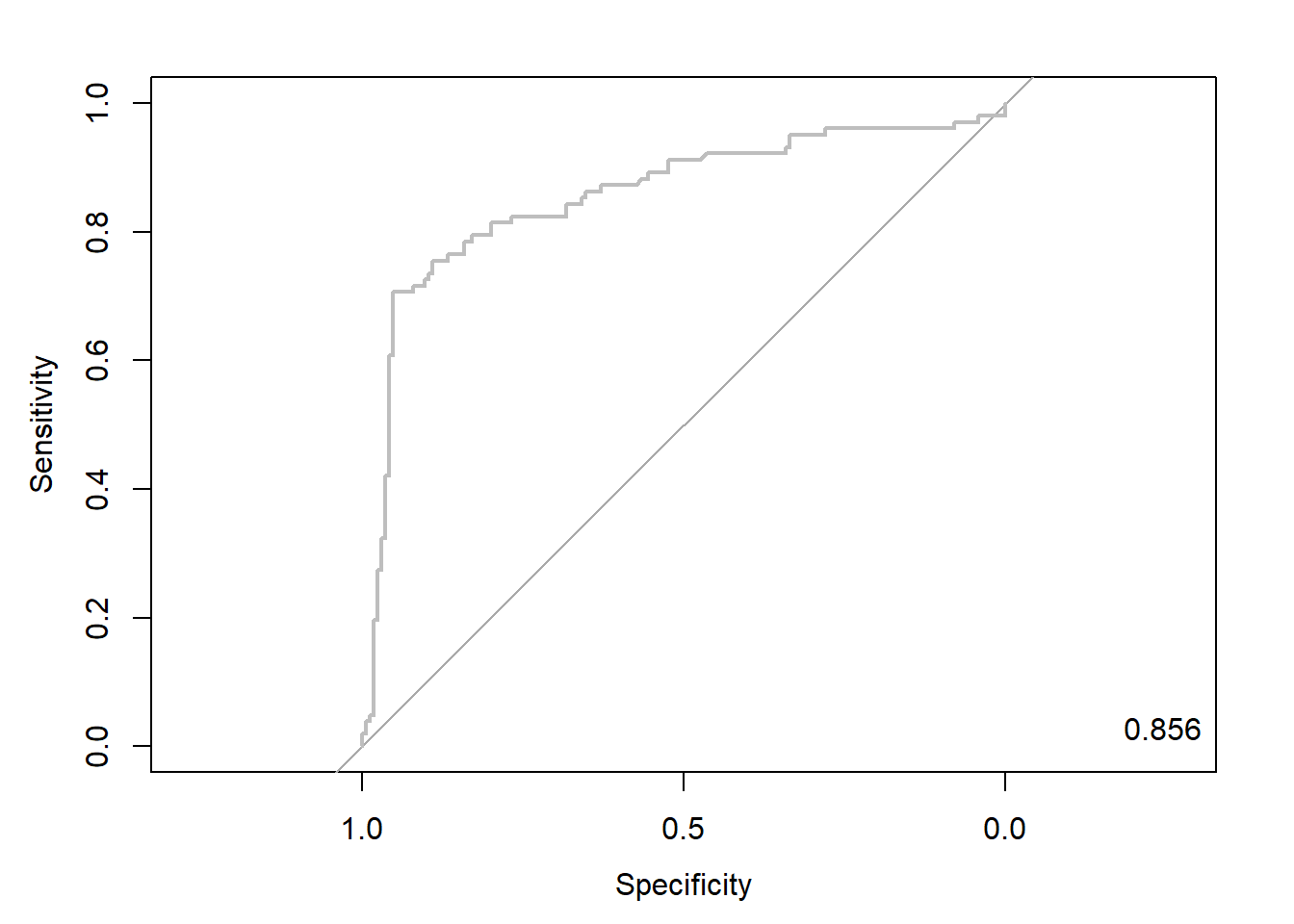
Caution! Package "pROC"를 통해 출력한 ROC 곡선은 다양한 함수를 이용해서 그래프를 수정할 수 있다.
# 함수 plot.roc() 이용
plot.roc(svm.roc,
         col="gray",                                        # Line Color
         print.auc = TRUE,                                  # AUC 출력 여부
         print.auc.col = "red",                             # AUC 글씨 색깔
         print.thres = TRUE,                                # Cutoff Value 출력 여부
         print.thres.pch = 19,                              # Cutoff Value를 표시하는 도형 모양
         print.thres.col = "red",                           # Cutoff Value를 표시하는 도형의 색깔
         auc.polygon = TRUE,                                # 곡선 아래 면적에 대한 여부
         auc.polygon.col = "gray90")                        # 곡선 아래 면적의 색깔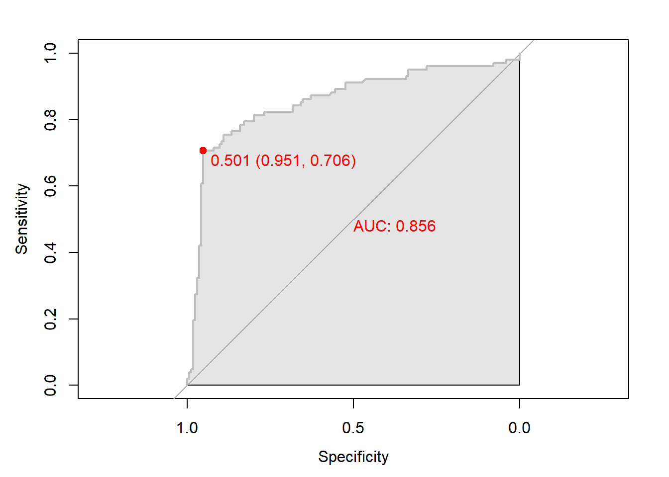
# 함수 ggroc() 이용
ggroc(svm.roc) +
annotate(geom = "text", x = 0.9, y = 1.0,
label = paste("AUC = ", auc),
size = 5,
color="red") +
theme_bw()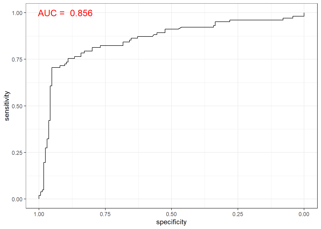
6.7.2.2 Package “Epi”
pacman::p_load("Epi")
# install_version("etm", version = "1.1", repos = "http://cran.us.r-project.org")

ROC(pp, ac, plot = "ROC") # ROC(예측 확률, 실제 class) 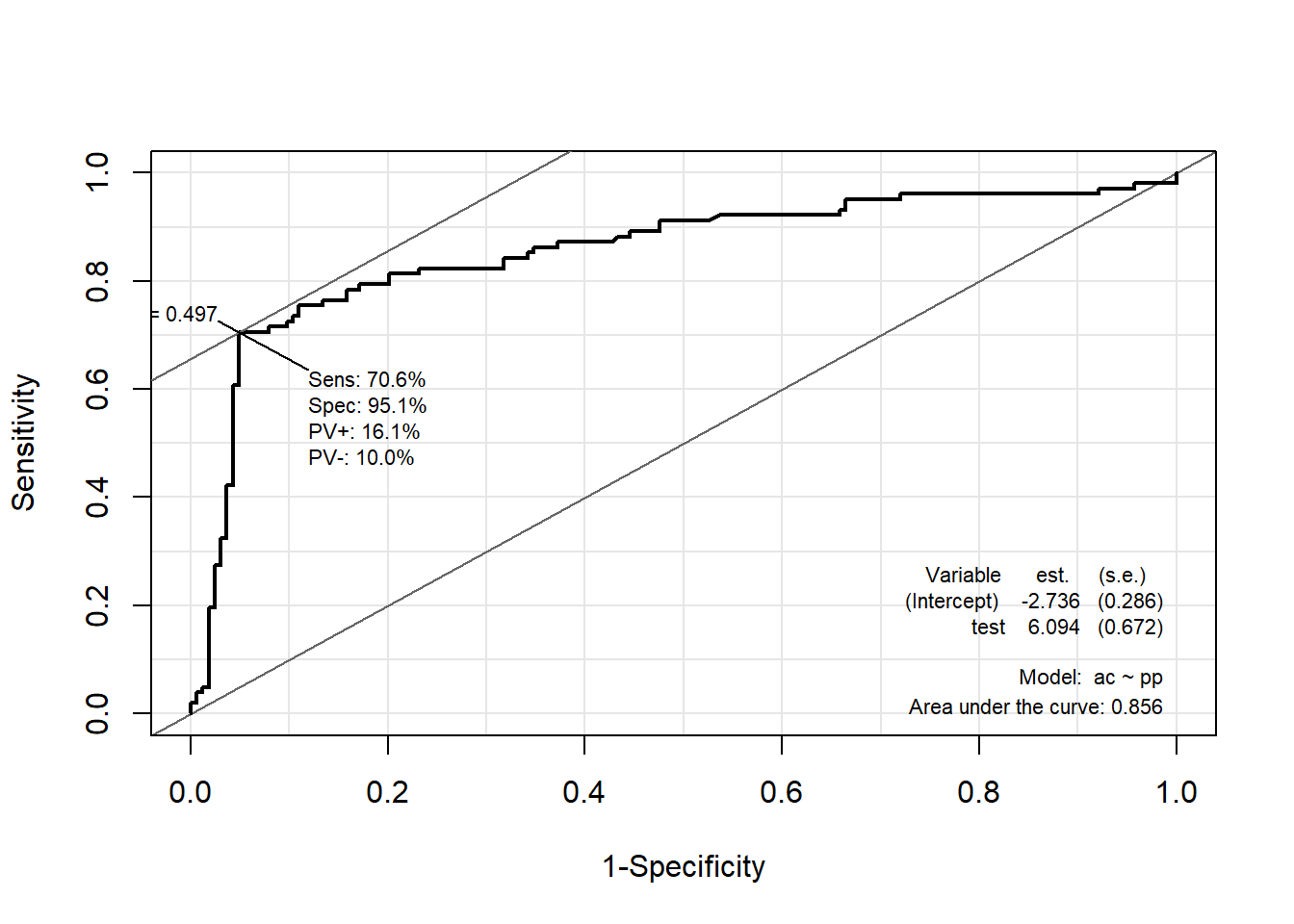
6.7.2.3 Package “ROCR”
pacman::p_load("ROCR")

svm.pred <- prediction(pp, ac)                              # prediction(예측 확률, 실제 class)

svm.perf <- performance(svm.pred, "tpr", "fpr")             # performance(, "민감도", "1-특이도")
plot(svm.perf, col = "gray")                                # ROC Curve

perf.auc   <- performance(svm.pred, "auc")                  # AUC
auc        <- attributes(perf.auc)$y.values
legend("bottomright", legend = auc, bty = "n")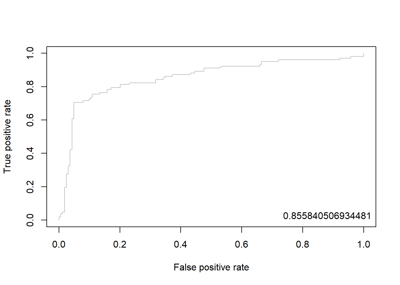
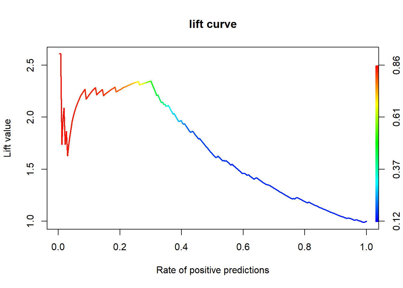
6.7.3 향상 차트
6.7.3.1 Package “ROCR”
svm.perf <- performance(svm.pred, "lift", "rpp")            # Lift Chart
plot(svm.perf, main = "lift curve",
     colorize = T,                                          # Coloring according to cutoff
     lwd = 2)