pacman::p_load("data.table",
               "tidyverse",
               "dplyr", "tidyr",
               "ggplot2", "GGally",
               "caret")

titanic <- fread("../Titanic.csv")                         # 데이터 불러오기

titanic %>%
as_tibble10 Logistic Regression
Logistic Regression의 장점
- 연속형 예측 변수와 범주형 예측 변수 모두 다룰 수 있다.
- 해석 가능한 모형이다.
- 예측 변수에 대해 정규분포 가정이 필요없다.
Logistic Regression의 단점
- 클래스가 완전히 분리되어 있는 경우에는 작동하지 않는다.
- 클래스에 대해 선형 분리를 가정하기 때문에 선형 분리가 불가능한 클래스 문제에는 성능이 좋지 않다.
- 각 예측 변수와 로그 오즈 간에 선형 관계를 가정하므로 어떤 예측 변수의 낮은 값과 높은 값이 동일한 클래스에 속한다면 중간 정도에 있는 값도 동일한 클래스에 속해야 한다.
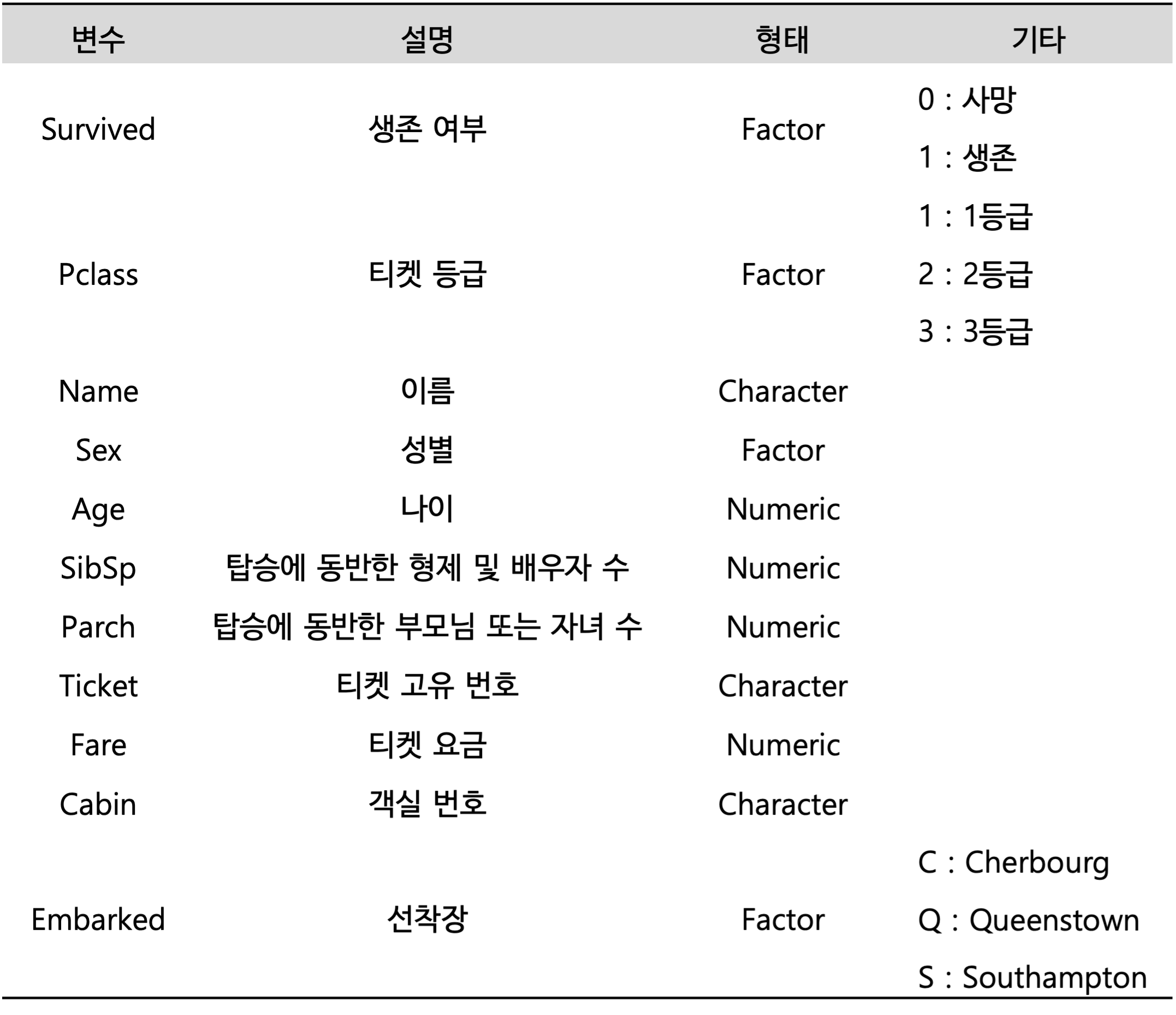
실습 자료 : 1912년 4월 15일 타이타닉호 침몰 당시 탑승객들의 정보를 기록한 데이터셋이며, 총 11개의 변수를 포함하고 있다. 이 자료에서 Target은
Survived이다.
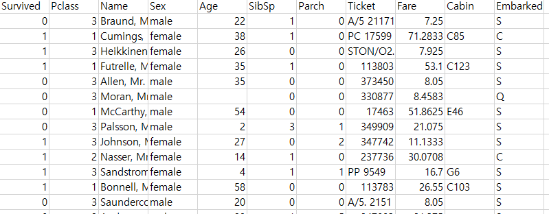
10.1 데이터 불러오기
# A tibble: 891 × 11
   Survived Pclass Name                                                Sex      Age SibSp Parch Ticket            Fare Cabin  Embarked
      <int>  <int> <chr>                                               <chr>  <dbl> <int> <int> <chr>            <dbl> <chr>  <chr>
 1        0      3 Braund, Mr. Owen Harris                             male      22     1     0 A/5 21171         7.25 ""     S
 2        1      1 Cumings, Mrs. John Bradley (Florence Briggs Thayer) female    38     1     0 PC 17599         71.3  "C85"  C
 3        1      3 Heikkinen, Miss. Laina                              female    26     0     0 STON/O2. 3101282  7.92 ""     S
 4        1      1 Futrelle, Mrs. Jacques Heath (Lily May Peel)        female    35     1     0 113803           53.1  "C123" S
 5        0      3 Allen, Mr. William Henry                            male      35     0     0 373450            8.05 ""     S
 6        0      3 Moran, Mr. James                                    male      NA     0     0 330877            8.46 ""     Q
 7        0      1 McCarthy, Mr. Timothy J                             male      54     0     0 17463            51.9  "E46"  S
 8        0      3 Palsson, Master. Gosta Leonard                      male       2     3     1 349909           21.1  ""     S
 9        1      3 Johnson, Mrs. Oscar W (Elisabeth Vilhelmina Berg)   female    27     0     2 347742           11.1  ""     S
10        1      2 Nasser, Mrs. Nicholas (Adele Achem)                 female    14     1     0 237736           30.1  ""     C
# ℹ 881 more rows
10.2 데이터 전처리 I
titanic %<>%
  data.frame() %>%                                                      # Data Frame 형태로 변환
  mutate(Survived = ifelse(Survived == 1, "yes", "no"))                 # Target을 문자형 변수로 변환

# 1. Convert to Factor
fac.col <- c("Pclass", "Sex",
             # Target
             "Survived")

titanic <- titanic %>%
  mutate_at(fac.col, as.factor)                                         # 범주형으로 변환

glimpse(titanic)                                                        # 데이터 구조 확인
Rows: 891
Columns: 11
$ Survived <fct> no, yes, yes, yes, no, no, no, no, yes, yes, yes, yes, no, no, no, yes, no, yes, no, yes, no, yes, yes, yes, no, yes, no, no, yes, no, no, yes, yes, no, no, no, yes, no, no, yes, no…
$ Pclass <fct> 3, 1, 3, 1, 3, 3, 1, 3, 3, 2, 3, 1, 3, 3, 3, 2, 3, 2, 3, 3, 2, 2, 3, 1, 3, 3, 3, 1, 3, 3, 1, 1, 3, 2, 1, 1, 3, 3, 3, 3, 3, 2, 3, 2, 3, 3, 3, 3, 3, 3, 3, 3, 1, 2, 1, 1, 2, 3, 2, 3, 3…
$ Name <chr> "Braund, Mr. Owen Harris", "Cumings, Mrs. John Bradley (Florence Briggs Thayer)", "Heikkinen, Miss. Laina", "Futrelle, Mrs. Jacques Heath (Lily May Peel)", "Allen, Mr. William Henry…
$ Sex <fct> male, female, female, female, male, male, male, male, female, female, female, female, male, male, female, female, male, male, female, female, male, male, female, male, female, femal…
$ Age <dbl> 22.0, 38.0, 26.0, 35.0, 35.0, NA, 54.0, 2.0, 27.0, 14.0, 4.0, 58.0, 20.0, 39.0, 14.0, 55.0, 2.0, NA, 31.0, NA, 35.0, 34.0, 15.0, 28.0, 8.0, 38.0, NA, 19.0, NA, NA, 40.0, NA, NA, 66.…
$ SibSp <int> 1, 1, 0, 1, 0, 0, 0, 3, 0, 1, 1, 0, 0, 1, 0, 0, 4, 0, 1, 0, 0, 0, 0, 0, 3, 1, 0, 3, 0, 0, 0, 1, 0, 0, 1, 1, 0, 0, 2, 1, 1, 1, 0, 1, 0, 0, 1, 0, 2, 1, 4, 0, 1, 1, 0, 0, 0, 0, 1, 5, 0…
$ Parch <int> 0, 0, 0, 0, 0, 0, 0, 1, 2, 0, 1, 0, 0, 5, 0, 0, 1, 0, 0, 0, 0, 0, 0, 0, 1, 5, 0, 2, 0, 0, 0, 0, 0, 0, 0, 0, 0, 0, 0, 0, 0, 0, 0, 2, 0, 0, 0, 0, 0, 0, 1, 0, 0, 0, 1, 0, 0, 0, 2, 2, 0…
$ Ticket <chr> "A/5 21171", "PC 17599", "STON/O2. 3101282", "113803", "373450", "330877", "17463", "349909", "347742", "237736", "PP 9549", "113783", "A/5. 2151", "347082", "350406", "248706", "38…
$ Fare <dbl> 7.2500, 71.2833, 7.9250, 53.1000, 8.0500, 8.4583, 51.8625, 21.0750, 11.1333, 30.0708, 16.7000, 26.5500, 8.0500, 31.2750, 7.8542, 16.0000, 29.1250, 13.0000, 18.0000, 7.2250, 26.0000,…
$ Cabin <chr> "", "C85", "", "C123", "", "", "E46", "", "", "", "G6", "C103", "", "", "", "", "", "", "", "", "", "D56", "", "A6", "", "", "", "C23 C25 C27", "", "", "", "B78", "", "", "", "", ""…
$ Embarked <chr> "S", "C", "S", "S", "S", "Q", "S", "S", "S", "C", "S", "S", "S", "S", "S", "S", "Q", "S", "S", "C", "S", "S", "Q", "S", "S", "S", "C", "S", "Q", "S", "C", "C", "Q", "S", "C", "S", "…# 2. Generate New Variable
titanic <- titanic %>%
mutate(FamSize = SibSp + Parch) # "FamSize = 형제 및 배우자 수 + 부모님 및 자녀 수"로 가족 수를 의미하는 새로운 변수
glimpse(titanic) # 데이터 구조 확인Rows: 891
Columns: 12
$ Survived <fct> no, yes, yes, yes, no, no, no, no, yes, yes, yes, yes, no, no, no, yes, no, yes, no, yes, no, yes, yes, yes, no, yes, no, no, yes, no, no, yes, yes, no, no, no, yes, no, no, yes, no…
$ Pclass <fct> 3, 1, 3, 1, 3, 3, 1, 3, 3, 2, 3, 1, 3, 3, 3, 2, 3, 2, 3, 3, 2, 2, 3, 1, 3, 3, 3, 1, 3, 3, 1, 1, 3, 2, 1, 1, 3, 3, 3, 3, 3, 2, 3, 2, 3, 3, 3, 3, 3, 3, 3, 3, 1, 2, 1, 1, 2, 3, 2, 3, 3…
$ Name <chr> "Braund, Mr. Owen Harris", "Cumings, Mrs. John Bradley (Florence Briggs Thayer)", "Heikkinen, Miss. Laina", "Futrelle, Mrs. Jacques Heath (Lily May Peel)", "Allen, Mr. William Henry…
$ Sex <fct> male, female, female, female, male, male, male, male, female, female, female, female, male, male, female, female, male, male, female, female, male, male, female, male, female, femal…
$ Age <dbl> 22.0, 38.0, 26.0, 35.0, 35.0, NA, 54.0, 2.0, 27.0, 14.0, 4.0, 58.0, 20.0, 39.0, 14.0, 55.0, 2.0, NA, 31.0, NA, 35.0, 34.0, 15.0, 28.0, 8.0, 38.0, NA, 19.0, NA, NA, 40.0, NA, NA, 66.…
$ SibSp <int> 1, 1, 0, 1, 0, 0, 0, 3, 0, 1, 1, 0, 0, 1, 0, 0, 4, 0, 1, 0, 0, 0, 0, 0, 3, 1, 0, 3, 0, 0, 0, 1, 0, 0, 1, 1, 0, 0, 2, 1, 1, 1, 0, 1, 0, 0, 1, 0, 2, 1, 4, 0, 1, 1, 0, 0, 0, 0, 1, 5, 0…
$ Parch <int> 0, 0, 0, 0, 0, 0, 0, 1, 2, 0, 1, 0, 0, 5, 0, 0, 1, 0, 0, 0, 0, 0, 0, 0, 1, 5, 0, 2, 0, 0, 0, 0, 0, 0, 0, 0, 0, 0, 0, 0, 0, 0, 0, 2, 0, 0, 0, 0, 0, 0, 1, 0, 0, 0, 1, 0, 0, 0, 2, 2, 0…
$ Ticket <chr> "A/5 21171", "PC 17599", "STON/O2. 3101282", "113803", "373450", "330877", "17463", "349909", "347742", "237736", "PP 9549", "113783", "A/5. 2151", "347082", "350406", "248706", "38…
$ Fare <dbl> 7.2500, 71.2833, 7.9250, 53.1000, 8.0500, 8.4583, 51.8625, 21.0750, 11.1333, 30.0708, 16.7000, 26.5500, 8.0500, 31.2750, 7.8542, 16.0000, 29.1250, 13.0000, 18.0000, 7.2250, 26.0000,…
$ Cabin <chr> "", "C85", "", "C123", "", "", "E46", "", "", "", "G6", "C103", "", "", "", "", "", "", "", "", "", "D56", "", "A6", "", "", "", "C23 C25 C27", "", "", "", "B78", "", "", "", "", ""…
$ Embarked <chr> "S", "C", "S", "S", "S", "Q", "S", "S", "S", "C", "S", "S", "S", "S", "S", "S", "Q", "S", "S", "C", "S", "S", "Q", "S", "S", "S", "C", "S", "Q", "S", "C", "C", "Q", "S", "C", "S", "…
$ FamSize <int> 1, 1, 0, 1, 0, 0, 0, 4, 2, 1, 2, 0, 0, 6, 0, 0, 5, 0, 1, 0, 0, 0, 0, 0, 4, 6, 0, 5, 0, 0, 0, 1, 0, 0, 1, 1, 0, 0, 2, 1, 1, 1, 0, 3, 0, 0, 1, 0, 2, 1, 5, 0, 1, 1, 1, 0, 0, 0, 3, 7, 0…# 3. Select Variables used for Analysis
titanic1 <- titanic %>%
select(Survived, Pclass, Sex, Age, Fare, FamSize) # 분석에 사용할 변수 선택
titanic1 %>%
as_tibble# A tibble: 891 × 6
Survived Pclass Sex Age Fare FamSize
<fct> <fct> <fct> <dbl> <dbl> <int>
1 no 3 male 22 7.25 1
2 yes 1 female 38 71.3 1
3 yes 3 female 26 7.92 0
4 yes 1 female 35 53.1 1
5 no 3 male 35 8.05 0
6 no 3 male NA 8.46 0
7 no 1 male 54 51.9 0
8 no 3 male 2 21.1 4
9 yes 3 female 27 11.1 2
10 yes 2 female 14 30.1 1
# ℹ 881 more rows10.3 데이터 탐색
ggpairs(titanic1,
        aes(colour = Survived)) +                         # Target의 범주에 따라 색깔을 다르게 표현
  theme_bw()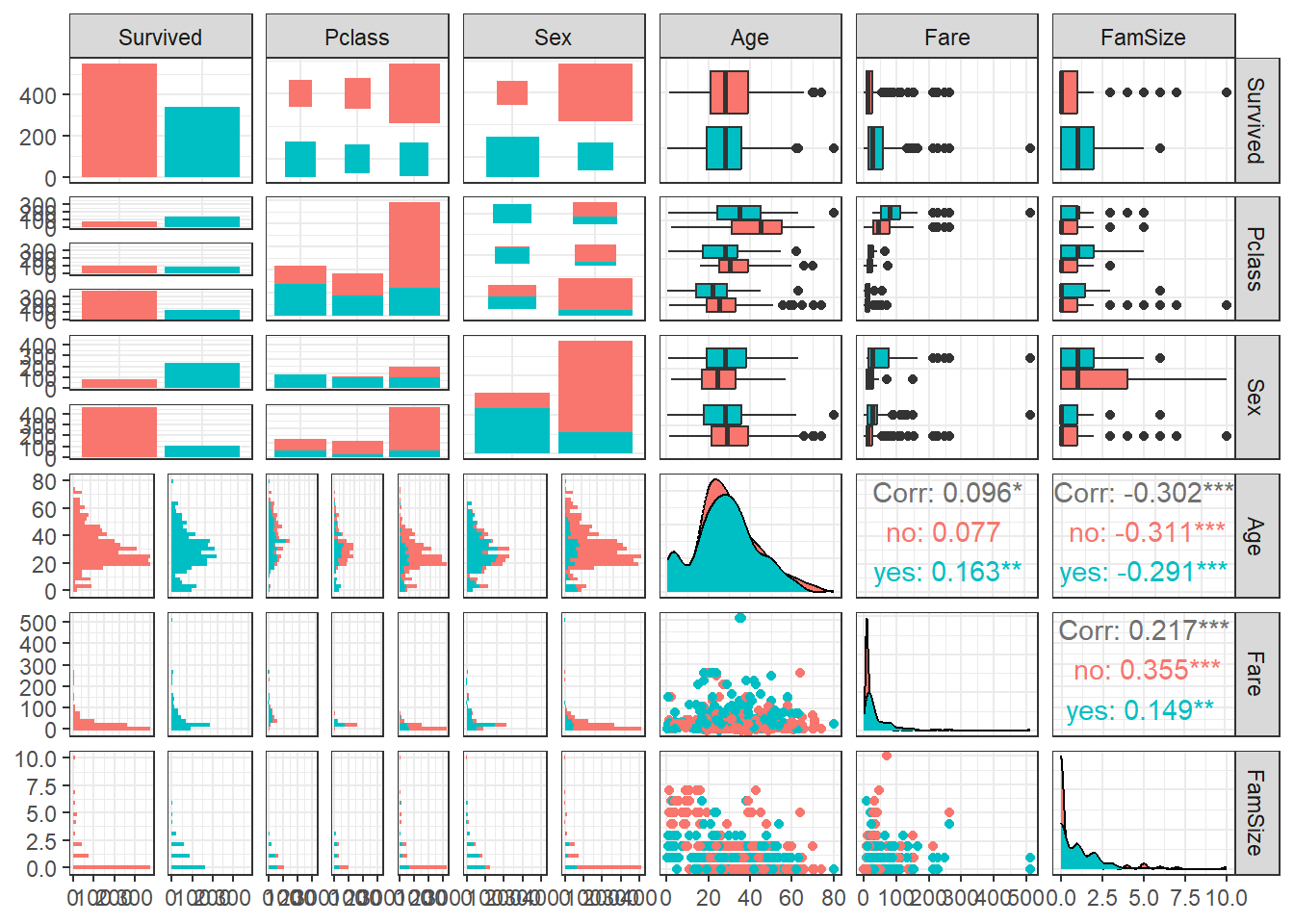
ggpairs(titanic1,
        aes(colour = Survived, alpha = 0.8)) +            # Target의 범주에 따라 색깔을 다르게 표현
  scale_colour_manual(values = c("purple", "cyan4")) +    # 특정 색깔 지정
  scale_fill_manual(values = c("purple", "cyan4")) +      # 특정 색깔 지정
  theme_bw()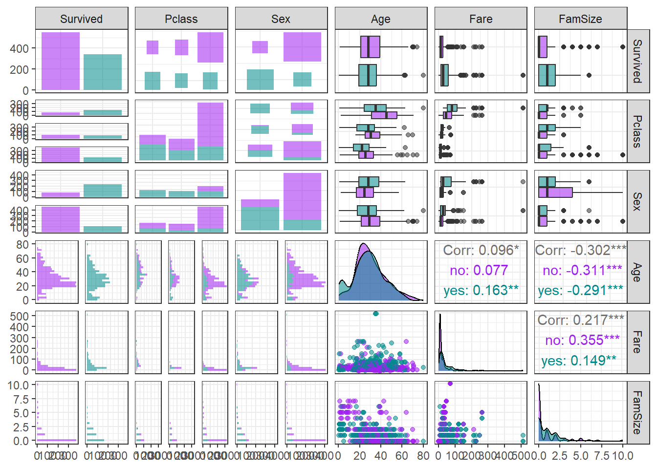
10.4 데이터 분할
# Partition (Training Dataset : Test Dataset = 7:3)
y      <- titanic1$Survived                             # Target

set.seed(200)
ind    <- createDataPartition(y, p = 0.7, list  =T)     # Index를 이용하여 7:3으로 분할
titanic.trd <- titanic1[ind$Resample1,]                 # Training Dataset
titanic.ted <- titanic1[-ind$Resample1,]                # Test Dataset
10.5 데이터 전처리 II
# 1. Imputation
titanic.trd.Imp <- titanic.trd %>%
  mutate(Age = replace_na(Age, mean(Age, na.rm = TRUE)))                 # 평균으로 결측값 대체

titanic.ted.Imp <- titanic.ted %>%
  mutate(Age = replace_na(Age, mean(titanic.trd$Age, na.rm = TRUE)))     # Training Dataset을 이용하여 결측값 대체

# 2. Standardization
preProcValues <- preProcess(titanic.trd.Imp,
                            method = c("center", "scale"))               # Standardization 정의 -> Training Dataset에 대한 평균과 표준편차 계산

titanic.trd.Imp <- predict(preProcValues, titanic.trd.Imp)               # Standardization for Training Dataset
titanic.ted.Imp <- predict(preProcValues, titanic.ted.Imp)               # Standardization for Test Dataset

glimpse(titanic.trd.Imp)                                                 # 데이터 구조 확인
Rows: 625
Columns: 6
$ Survived <fct> no, yes, yes, no, no, no, yes, yes, yes, yes, no, no, yes, no, yes, no, yes, no, no, no, yes, no, no, yes, yes, no, no, no, no, no, yes, no, no, no, yes, no, yes, no, no, no, yes, n…
$ Pclass <fct> 3, 3, 1, 3, 3, 3, 3, 2, 3, 1, 3, 3, 2, 3, 3, 2, 1, 3, 3, 1, 3, 3, 1, 1, 3, 2, 1, 1, 3, 3, 3, 3, 2, 3, 3, 3, 3, 3, 3, 3, 1, 1, 1, 3, 3, 1, 3, 1, 3, 3, 3, 3, 3, 3, 2, 3, 3, 3, 1, 2, 3…
$ Sex <fct> male, female, female, male, male, male, female, female, female, female, male, female, male, female, female, male, male, female, male, male, female, male, male, female, female, male,…
$ Age <dbl> -0.61306970, -0.30411628, 0.39102893, 0.39102893, 0.00000000, -2.15783684, -0.22687792, -1.23097656, -2.00336012, 2.16751113, 0.69998236, -1.23097656, 0.00000000, 0.08207551, 0.0000…
$ Fare <dbl> -0.51776394, -0.50463325, 0.37414970, -0.50220165, -0.49425904, -0.24882814, -0.44222264, -0.07383411, -0.33393441, -0.14232374, -0.05040897, -0.50601052, -0.40590999, -0.30864569, …
$ FamSize <dbl> 0.04506631, -0.55421976, 0.04506631, -0.55421976, -0.55421976, 1.84292454, 0.64435239, 0.04506631, 0.64435239, -0.55421976, 3.04149669, -0.55421976, -0.55421976, 0.04506631, -0.5542…glimpse(titanic.ted.Imp) # 데이터 구조 확인Rows: 266
Columns: 6
$ Survived <fct> yes, no, no, yes, no, yes, yes, yes, yes, yes, no, no, yes, yes, no, yes, no, yes, yes, no, yes, no, no, no, no, no, no, yes, yes, no, no, no, no, no, no, no, no, no, no, yes, no, n…
$ Pclass <fct> 1, 1, 3, 2, 3, 2, 3, 3, 3, 2, 3, 3, 2, 2, 3, 2, 1, 3, 2, 3, 3, 2, 2, 3, 3, 3, 3, 1, 2, 2, 3, 3, 3, 3, 3, 2, 3, 2, 2, 2, 3, 3, 2, 1, 3, 1, 3, 2, 1, 3, 3, 3, 3, 3, 3, 3, 3, 1, 3, 1, 3…
$ Sex <fct> female, male, male, female, male, male, female, female, male, female, male, male, female, female, male, female, male, male, female, male, female, male, male, male, male, male, male,…
$ Age <dbl> 0.62274400, 1.85855771, -0.76754642, 1.93579607, -2.15783684, 0.31379058, -1.15373820, 0.62274400, 0.00000000, -2.08059848, 0.00000000, -0.69030806, -0.07240121, -0.69030806, -0.111…
$ Fare <dbl> 0.727866891, 0.350076786, -0.502201647, -0.347551409, -0.092232621, -0.405909990, -0.502606266, -0.048220525, -0.518168555, 0.150037190, -0.502201647, -0.507064862, -0.153022808, -0…
$ FamSize <dbl> 0.04506631, -0.55421976, -0.55421976, -0.55421976, 2.44221062, -0.55421976, -0.55421976, 3.04149669, -0.55421976, 1.24363847, -0.55421976, -0.55421976, 0.04506631, -0.55421976, -0.5…10.6 모형 훈련
Caution! 함수 glm()에서 Logistic Regression은 Target이 2개의 클래스를 가질 때 “두 번째 클래스”에 속할 확률을 모델링하며, 범주형 예측 변수의 경우 더미 변환을 자동적으로 수행한다. 여기서, “두 번째 클래스”란 “Factor” 변환하였을 때 두 번째 수준(Level)을 의미한다. 예를 들어, “a”와 “b” 2개의 클래스를 가진 Target을 “Factor” 변환하였을 때 수준이 “a” “b”라면, 첫 번째 클래스는 “a”, 두 번째 클래스는 “b”가 된다.
logis.fit <- glm(Survived ~ . , data = titanic.trd.Imp,
                 family = "binomial")                  # For Logit Transformation

logis.fit                                              # Fitted Logistic Regression
Call:  glm(formula = Survived ~ ., family = "binomial", data = titanic.trd.Imp)

Coefficients:
(Intercept)      Pclass2      Pclass3      Sexmale          Age         Fare      FamSize
     2.5729      -1.0518      -2.3731      -2.7202      -0.5296       0.1226      -0.3978

Degrees of Freedom: 624 Total (i.e. Null);  618 Residual
Null Deviance:      832.5
Residual Deviance: 555.1 AIC: 569.1summary(logis.fit) # Summary for Fitted Logistic Regression
Call:
glm(formula = Survived ~ ., family = "binomial", data = titanic.trd.Imp)

Deviance Residuals:
    Min       1Q   Median       3Q      Max
-2.6575  -0.6298  -0.4076   0.6127   2.4606

Coefficients:
            Estimate Std. Error z value Pr(>|z|)
(Intercept)   2.5729     0.3141   8.192 2.58e-16 ***
Pclass2      -1.0518     0.3546  -2.966  0.00302 **
Pclass3      -2.3731     0.3477  -6.826 8.76e-12 ***
Sexmale      -2.7202     0.2390 -11.381  < 2e-16 ***
Age          -0.5296     0.1207  -4.386 1.15e-05 ***
Fare          0.1226     0.1499   0.818  0.41351
FamSize      -0.3978     0.1356  -2.934  0.00335 **
---
Signif. codes:  0 '***' 0.001 '**' 0.01 '*' 0.05 '.' 0.1 ' ' 1

(Dispersion parameter for binomial family taken to be 1)

    Null deviance: 832.49  on 624  degrees of freedom
Residual deviance: 555.06  on 618  degrees of freedom
AIC: 569.06

Number of Fisher Scoring iterations: 5
Result! 데이터 “titanic.trd.Imp”의 Target “Survived”은 “no”와 “yes” 2개의 클래스를 가지며, “Factor” 변환하면 알파벳순으로 수준을 부여하기 때문에 “yes”가 두 번째 클래스가 된다. 즉, “yes”에 속할 확률(= 탑승객이 생존할 확률)을 \(p\)라고 할 때, 추정된 회귀계수를 이용하여 다음과 같은 모형식을 얻을 수 있다. \[
\begin{align*}
\log{\frac{p}{1-p}} = &\;2.573 - 1.052X_{\text{Pclass2}} - 2.373 X_{\text{Pclass3}} -2.720 X_{\text{Sexmale}} \\
&-0.530 Z_{\text{Age}} +0.123 Z_{\text{Fare}} - 0.398 Z_{\text{FamSize}}
\end{align*}
\] 여기서, \(Z_{\text{예측 변수}}\)는 표준화한 예측 변수, \(X_{\text{예측 변수}}\)는 더미 변수를 의미한다.
범주형 예측 변수(“Pclass”, “Sex”)는 더미 변환이 수행되었는데, 예를 들어, \(X_{\text{Pclass2}}\)는 탑승객의 티켓 등급이 2등급인 경우 “1”값을 가지고 2등급이 아니면 “0”값을 가진다.
OR <- exp(coef(logis.fit))                             # Odds Ratio
CI <- exp(confint(logis.fit))                          # 95% Confidence Interval

cbind("Odds Ratio" = round(OR, 3),                     # round : 반올림
      round(CI, 3))
Odds Ratio 2.5 % 97.5 %
(Intercept) 13.104 7.159 24.579
Pclass2 0.349 0.173 0.698
Pclass3 0.093 0.047 0.184
Sexmale 0.066 0.041 0.104
Age 0.589 0.462 0.743
Fare 1.130 0.858 1.571
FamSize 0.672 0.507 0.865Result! 오즈비를 살펴보면, 나이(“Age”)를 표준화한 값이 1 증가할 경우, 탑승객의 생존 가능성은 1.700(=1/0.589)배 감소한다. 반면, 티켓 요금(“Fare”)을 표준화한 값이 1 증가할 경우, 탑승객의 생존 가능성은 1.130배 증가한다.
10.7 모형 평가
Caution! 모형 평가를 위해 Test Dataset에 대한 예측 class/확률 이 필요하며, 함수 predict()를 이용하여 생성한다.
# 예측 확률 생성
test.logis.prob <- predict(logis.fit,
                           newdata = titanic.ted.Imp,                      # Test Dataset including Only 예측 변수
                           type = "response")                              # 예측 확률 생성

test.logis.prob %>%                                                        # "Survived = yes"에 대한 예측 확률
  as_tibble
# A tibble: 266 × 1
value
<dbl>
1 0.910
2 0.296
3 0.124
4 0.662
5 0.0862
6 0.232
7 0.725
8 0.207
9 0.0860
10 0.895
# ℹ 256 more rows# 예측 class 생성
logis.pred <- ifelse(test.logis.prob > 0.5, "yes", "no") %>% # "Survived = yes"에 대한 예측 확률이 0.5 초과하면 "yes", 0.5를 넘기지 못하면 "no"로 분류
factor # 범주형으로 변환
logis.pred %>%
as_tibble# A tibble: 266 × 1
value
<fct>
1 yes
2 no
3 no
4 yes
5 no
6 no
7 yes
8 no
9 no
10 yes
# ℹ 256 more rows10.7.1 ConfusionMatrix
CM   <- caret::confusionMatrix(logis.pred, titanic.ted.Imp$Survived,
                               positive = "yes")        # confusionMatrix(예측 class, 실제 class, positive = "관심 class")
CM
Confusion Matrix and Statistics
Reference
Prediction no yes
no 148 32
yes 16 70
Accuracy : 0.8195
95% CI : (0.768, 0.8638)
No Information Rate : 0.6165
P-Value [Acc > NIR] : 5.675e-13
Kappa : 0.6067
Mcnemar's Test P-Value : 0.03038
Sensitivity : 0.6863
Specificity : 0.9024
Pos Pred Value : 0.8140
Neg Pred Value : 0.8222
Prevalence : 0.3835
Detection Rate : 0.2632
Detection Prevalence : 0.3233
Balanced Accuracy : 0.7944
'Positive' Class : yes
10.7.2 ROC 곡선
ac  <- titanic.ted.Imp$Survived                           # Test Dataset의 실제 class
pp  <- as.numeric(test.logis.prob)                        # 예측 확률을 수치형으로 변환
10.7.2.1 Package “pROC”
pacman::p_load("pROC")

logis.roc  <- roc(ac, pp, plot = T, col = "gray")         # roc(실제 class, 예측 확률)
auc        <- round(auc(logis.roc), 3)
legend("bottomright", legend = auc, bty = "n")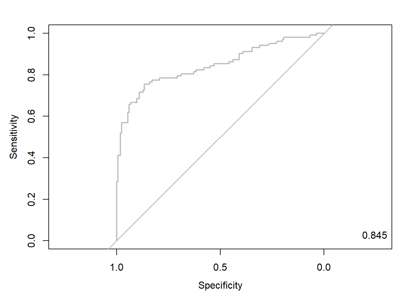
Caution! Package "pROC"를 통해 출력한 ROC 곡선은 다양한 함수를 이용해서 그래프를 수정할 수 있다.
# 함수 plot.roc() 이용
plot.roc(logis.roc,
         col="gray",                                      # Line Color
         print.auc = TRUE,                                # AUC 출력 여부
         print.auc.col = "red",                           # AUC 글씨 색깔
         print.thres = TRUE,                              # Cutoff Value 출력 여부
         print.thres.pch = 19,                            # Cutoff Value를 표시하는 도형 모양
         print.thres.col = "red",                         # Cutoff Value를 표시하는 도형의 색깔
         auc.polygon = TRUE,                              # 곡선 아래 면적에 대한 여부
         auc.polygon.col = "gray90")                      # 곡선 아래 면적의 색깔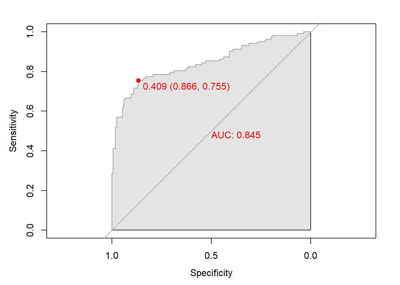
# 함수 ggroc() 이용
ggroc(logis.roc) +
annotate(geom = "text", x = 0.9, y = 1.0,
label = paste("AUC = ", auc),
size = 5,
color="red") +
theme_bw()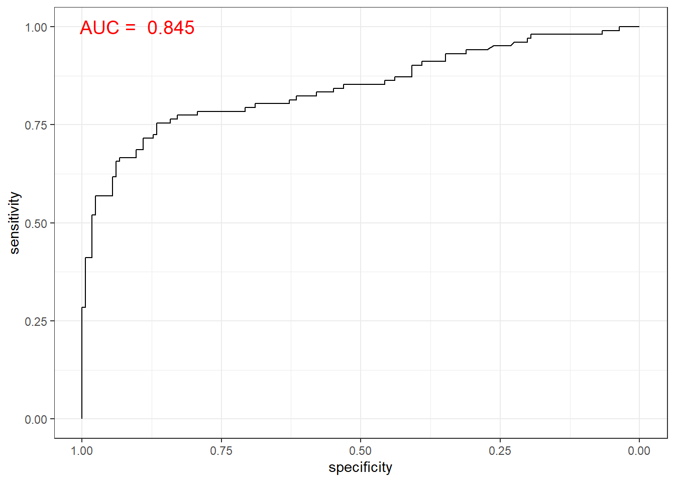
10.7.2.2 Package “Epi”
pacman::p_load("Epi")
# install_version("etm", version = "1.1", repos = "http://cran.us.r-project.org")

ROC(pp, ac, plot = "ROC") # ROC(예측 확률, 실제 class) 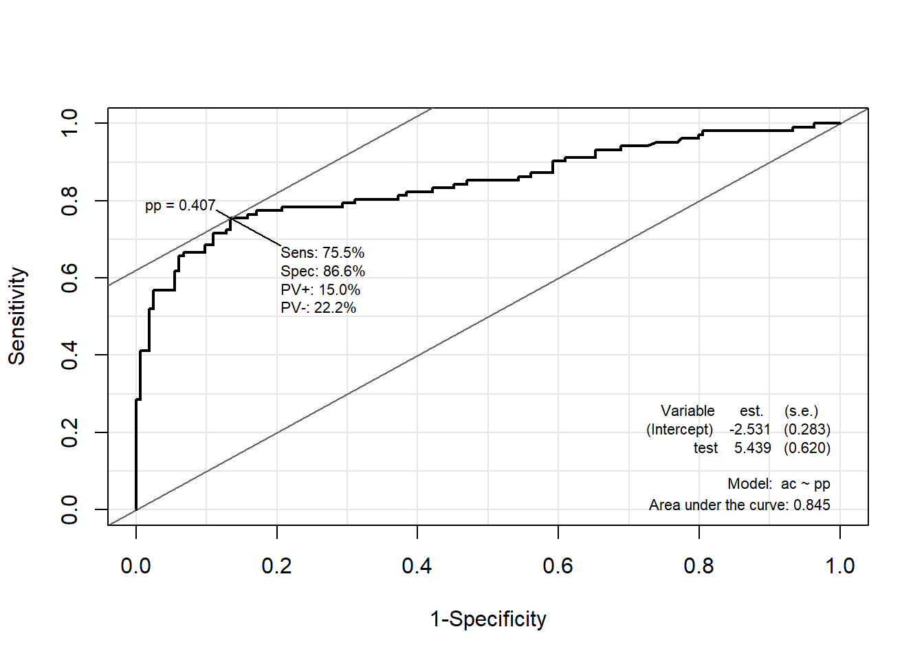
10.7.2.3 Package “ROCR”
pacman::p_load("ROCR")

logis.pred <- prediction(pp, ac)                          # prediction(예측 확률, 실제 class)

logis.perf <- performance(logis.pred, "tpr", "fpr")       # performance(, "민감도", "1-특이도")
plot(logis.perf, col = "gray")                            # ROC Curve

perf.auc   <- performance(logis.pred, "auc")              # AUC
auc        <- attributes(perf.auc)$y.values
legend("bottomright", legend = auc, bty = "n")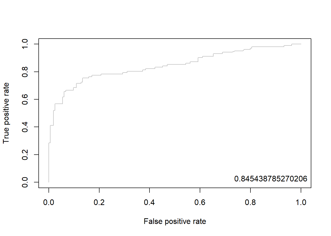
10.7.3 향상 차트
10.7.3.1 Package “ROCR”
logis.pred <- performance(logis.pred, "lift", "rpp")      # Lift Chart
plot(logis.pred, main = "lift curve",
     colorize = T,                                        # Coloring according to cutoff
lwd = 2) 