pacman::p_load("data.table",
               "tidyverse",
               "dplyr", "tidyr",
               "ggplot2", "GGally",
               "caret",
               "doParallel", "parallel")                                # For 병렬 처리

registerDoParallel(cores=detectCores())                                 # 사용할 Core 개수 지정

titanic <- fread("../Titanic.csv")                                      # 데이터 불러오기

titanic %>%
as_tibble9 Elastic Net Regression
Elastic Net Regression의 장점
- 예측 변수의 개수가 표본의 크기보다 큰 경우,
LASSO Regression의 문제(표본의 크기보다 많은 예측 변수를 선택 X)를 극복한다. - 예측 변수 사이에 어떤 그룹 구조(쌍별 상관 관계가 매우 높은)가 있을 때,
LASSO Regression의 문제(그룹에서 하나의 예측 변수만 선택)를 극복한다.
Elastic Net Regression의 단점
Ridge Regression이나LASSO Regression에 매우 근접하지 않을 경우, 만족스럽지 않은 결과를 보여준다.- 이중 수축 문제(Double Shrinkage Problem)가 발생한다.
Ridge Regression이나LASSO Regression에 비해 분산을 크게 줄이는 데 도움이 되지 않고, 불필요한 편의(bias)가 추가로 발생한다.
- 회귀계수에 대한 추정치만 계산이 가능하며, 회귀계수에 대한 추론(신뢰 구간 등)은 불가능하다.
실습 자료 : 1912년 4월 15일 타이타닉호 침몰 당시 탑승객들의 정보를 기록한 데이터셋이며, 총 11개의 변수를 포함하고 있다. 이 자료에서 Target은
Survived이다.
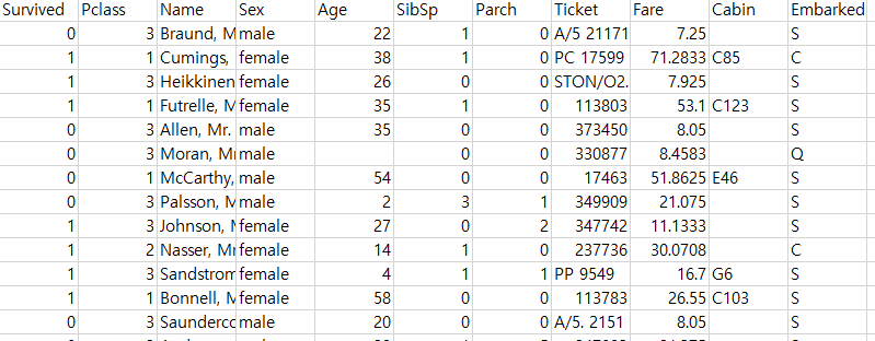

9.1 데이터 불러오기
# A tibble: 891 × 11
   Survived Pclass Name                                                Sex      Age SibSp Parch Ticket            Fare Cabin  Embarked
      <int>  <int> <chr>                                               <chr>  <dbl> <int> <int> <chr>            <dbl> <chr>  <chr>
 1        0      3 Braund, Mr. Owen Harris                             male      22     1     0 A/5 21171         7.25 ""     S
 2        1      1 Cumings, Mrs. John Bradley (Florence Briggs Thayer) female    38     1     0 PC 17599         71.3  "C85"  C
 3        1      3 Heikkinen, Miss. Laina                              female    26     0     0 STON/O2. 3101282  7.92 ""     S
 4        1      1 Futrelle, Mrs. Jacques Heath (Lily May Peel)        female    35     1     0 113803           53.1  "C123" S
 5        0      3 Allen, Mr. William Henry                            male      35     0     0 373450            8.05 ""     S
 6        0      3 Moran, Mr. James                                    male      NA     0     0 330877            8.46 ""     Q
 7        0      1 McCarthy, Mr. Timothy J                             male      54     0     0 17463            51.9  "E46"  S
 8        0      3 Palsson, Master. Gosta Leonard                      male       2     3     1 349909           21.1  ""     S
 9        1      3 Johnson, Mrs. Oscar W (Elisabeth Vilhelmina Berg)   female    27     0     2 347742           11.1  ""     S
10        1      2 Nasser, Mrs. Nicholas (Adele Achem)                 female    14     1     0 237736           30.1  ""     C
# ℹ 881 more rows
9.2 데이터 전처리
titanic %<>%
  data.frame() %>%                                                      # Data Frame 형태로 변환
  mutate(Survived = ifelse(Survived == 1, "yes", "no"))                 # Target을 문자형 변수로 변환

# 1. Convert to Factor
fac.col <- c("Pclass", "Sex",
             # Target
             "Survived")

titanic <- titanic %>%
  mutate_at(fac.col, as.factor)                                         # 범주형으로 변환

glimpse(titanic)                                                        # 데이터 구조 확인
Rows: 891
Columns: 11
$ Survived <fct> no, yes, yes, yes, no, no, no, no, yes, yes, yes, yes, no, no, no, yes, no, yes, no, yes, no, yes, yes, yes, no, yes, no, no, yes, no, no, yes, yes, no, no, no, yes, no, no, yes, no…
$ Pclass <fct> 3, 1, 3, 1, 3, 3, 1, 3, 3, 2, 3, 1, 3, 3, 3, 2, 3, 2, 3, 3, 2, 2, 3, 1, 3, 3, 3, 1, 3, 3, 1, 1, 3, 2, 1, 1, 3, 3, 3, 3, 3, 2, 3, 2, 3, 3, 3, 3, 3, 3, 3, 3, 1, 2, 1, 1, 2, 3, 2, 3, 3…
$ Name <chr> "Braund, Mr. Owen Harris", "Cumings, Mrs. John Bradley (Florence Briggs Thayer)", "Heikkinen, Miss. Laina", "Futrelle, Mrs. Jacques Heath (Lily May Peel)", "Allen, Mr. William Henry…
$ Sex <fct> male, female, female, female, male, male, male, male, female, female, female, female, male, male, female, female, male, male, female, female, male, male, female, male, female, femal…
$ Age <dbl> 22.0, 38.0, 26.0, 35.0, 35.0, NA, 54.0, 2.0, 27.0, 14.0, 4.0, 58.0, 20.0, 39.0, 14.0, 55.0, 2.0, NA, 31.0, NA, 35.0, 34.0, 15.0, 28.0, 8.0, 38.0, NA, 19.0, NA, NA, 40.0, NA, NA, 66.…
$ SibSp <int> 1, 1, 0, 1, 0, 0, 0, 3, 0, 1, 1, 0, 0, 1, 0, 0, 4, 0, 1, 0, 0, 0, 0, 0, 3, 1, 0, 3, 0, 0, 0, 1, 0, 0, 1, 1, 0, 0, 2, 1, 1, 1, 0, 1, 0, 0, 1, 0, 2, 1, 4, 0, 1, 1, 0, 0, 0, 0, 1, 5, 0…
$ Parch <int> 0, 0, 0, 0, 0, 0, 0, 1, 2, 0, 1, 0, 0, 5, 0, 0, 1, 0, 0, 0, 0, 0, 0, 0, 1, 5, 0, 2, 0, 0, 0, 0, 0, 0, 0, 0, 0, 0, 0, 0, 0, 0, 0, 2, 0, 0, 0, 0, 0, 0, 1, 0, 0, 0, 1, 0, 0, 0, 2, 2, 0…
$ Ticket <chr> "A/5 21171", "PC 17599", "STON/O2. 3101282", "113803", "373450", "330877", "17463", "349909", "347742", "237736", "PP 9549", "113783", "A/5. 2151", "347082", "350406", "248706", "38…
$ Fare <dbl> 7.2500, 71.2833, 7.9250, 53.1000, 8.0500, 8.4583, 51.8625, 21.0750, 11.1333, 30.0708, 16.7000, 26.5500, 8.0500, 31.2750, 7.8542, 16.0000, 29.1250, 13.0000, 18.0000, 7.2250, 26.0000,…
$ Cabin <chr> "", "C85", "", "C123", "", "", "E46", "", "", "", "G6", "C103", "", "", "", "", "", "", "", "", "", "D56", "", "A6", "", "", "", "C23 C25 C27", "", "", "", "B78", "", "", "", "", ""…
$ Embarked <chr> "S", "C", "S", "S", "S", "Q", "S", "S", "S", "C", "S", "S", "S", "S", "S", "S", "Q", "S", "S", "C", "S", "S", "Q", "S", "S", "S", "C", "S", "Q", "S", "C", "C", "Q", "S", "C", "S", "…# 2. Generate New Variable
titanic <- titanic %>%
mutate(FamSize = SibSp + Parch) # "FamSize = 형제 및 배우자 수 + 부모님 및 자녀 수"로 가족 수를 의미하는 새로운 변수
glimpse(titanic) # 데이터 구조 확인Rows: 891
Columns: 12
$ Survived <fct> no, yes, yes, yes, no, no, no, no, yes, yes, yes, yes, no, no, no, yes, no, yes, no, yes, no, yes, yes, yes, no, yes, no, no, yes, no, no, yes, yes, no, no, no, yes, no, no, yes, no…
$ Pclass <fct> 3, 1, 3, 1, 3, 3, 1, 3, 3, 2, 3, 1, 3, 3, 3, 2, 3, 2, 3, 3, 2, 2, 3, 1, 3, 3, 3, 1, 3, 3, 1, 1, 3, 2, 1, 1, 3, 3, 3, 3, 3, 2, 3, 2, 3, 3, 3, 3, 3, 3, 3, 3, 1, 2, 1, 1, 2, 3, 2, 3, 3…
$ Name <chr> "Braund, Mr. Owen Harris", "Cumings, Mrs. John Bradley (Florence Briggs Thayer)", "Heikkinen, Miss. Laina", "Futrelle, Mrs. Jacques Heath (Lily May Peel)", "Allen, Mr. William Henry…
$ Sex <fct> male, female, female, female, male, male, male, male, female, female, female, female, male, male, female, female, male, male, female, female, male, male, female, male, female, femal…
$ Age <dbl> 22.0, 38.0, 26.0, 35.0, 35.0, NA, 54.0, 2.0, 27.0, 14.0, 4.0, 58.0, 20.0, 39.0, 14.0, 55.0, 2.0, NA, 31.0, NA, 35.0, 34.0, 15.0, 28.0, 8.0, 38.0, NA, 19.0, NA, NA, 40.0, NA, NA, 66.…
$ SibSp <int> 1, 1, 0, 1, 0, 0, 0, 3, 0, 1, 1, 0, 0, 1, 0, 0, 4, 0, 1, 0, 0, 0, 0, 0, 3, 1, 0, 3, 0, 0, 0, 1, 0, 0, 1, 1, 0, 0, 2, 1, 1, 1, 0, 1, 0, 0, 1, 0, 2, 1, 4, 0, 1, 1, 0, 0, 0, 0, 1, 5, 0…
$ Parch <int> 0, 0, 0, 0, 0, 0, 0, 1, 2, 0, 1, 0, 0, 5, 0, 0, 1, 0, 0, 0, 0, 0, 0, 0, 1, 5, 0, 2, 0, 0, 0, 0, 0, 0, 0, 0, 0, 0, 0, 0, 0, 0, 0, 2, 0, 0, 0, 0, 0, 0, 1, 0, 0, 0, 1, 0, 0, 0, 2, 2, 0…
$ Ticket <chr> "A/5 21171", "PC 17599", "STON/O2. 3101282", "113803", "373450", "330877", "17463", "349909", "347742", "237736", "PP 9549", "113783", "A/5. 2151", "347082", "350406", "248706", "38…
$ Fare <dbl> 7.2500, 71.2833, 7.9250, 53.1000, 8.0500, 8.4583, 51.8625, 21.0750, 11.1333, 30.0708, 16.7000, 26.5500, 8.0500, 31.2750, 7.8542, 16.0000, 29.1250, 13.0000, 18.0000, 7.2250, 26.0000,…
$ Cabin <chr> "", "C85", "", "C123", "", "", "E46", "", "", "", "G6", "C103", "", "", "", "", "", "", "", "", "", "D56", "", "A6", "", "", "", "C23 C25 C27", "", "", "", "B78", "", "", "", "", ""…
$ Embarked <chr> "S", "C", "S", "S", "S", "Q", "S", "S", "S", "C", "S", "S", "S", "S", "S", "S", "Q", "S", "S", "C", "S", "S", "Q", "S", "S", "S", "C", "S", "Q", "S", "C", "C", "Q", "S", "C", "S", "…
$ FamSize <int> 1, 1, 0, 1, 0, 0, 0, 4, 2, 1, 2, 0, 0, 6, 0, 0, 5, 0, 1, 0, 0, 0, 0, 0, 4, 6, 0, 5, 0, 0, 0, 1, 0, 0, 1, 1, 0, 0, 2, 1, 1, 1, 0, 3, 0, 0, 1, 0, 2, 1, 5, 0, 1, 1, 1, 0, 0, 0, 3, 7, 0…# 3. Select Variables used for Analysis
titanic1 <- titanic %>%
select(Survived, Pclass, Sex, Age, Fare, FamSize) # 분석에 사용할 변수 선택
titanic1 %>%
as_tibble# A tibble: 891 × 6
Survived Pclass Sex Age Fare FamSize
<fct> <fct> <fct> <dbl> <dbl> <int>
1 no 3 male 22 7.25 1
2 yes 1 female 38 71.3 1
3 yes 3 female 26 7.92 0
4 yes 1 female 35 53.1 1
5 no 3 male 35 8.05 0
6 no 3 male NA 8.46 0
7 no 1 male 54 51.9 0
8 no 3 male 2 21.1 4
9 yes 3 female 27 11.1 2
10 yes 2 female 14 30.1 1
# ℹ 881 more rows9.3 데이터 탐색
ggpairs(titanic1,
        aes(colour = Survived)) +                         # Target의 범주에 따라 색깔을 다르게 표현
  theme_bw()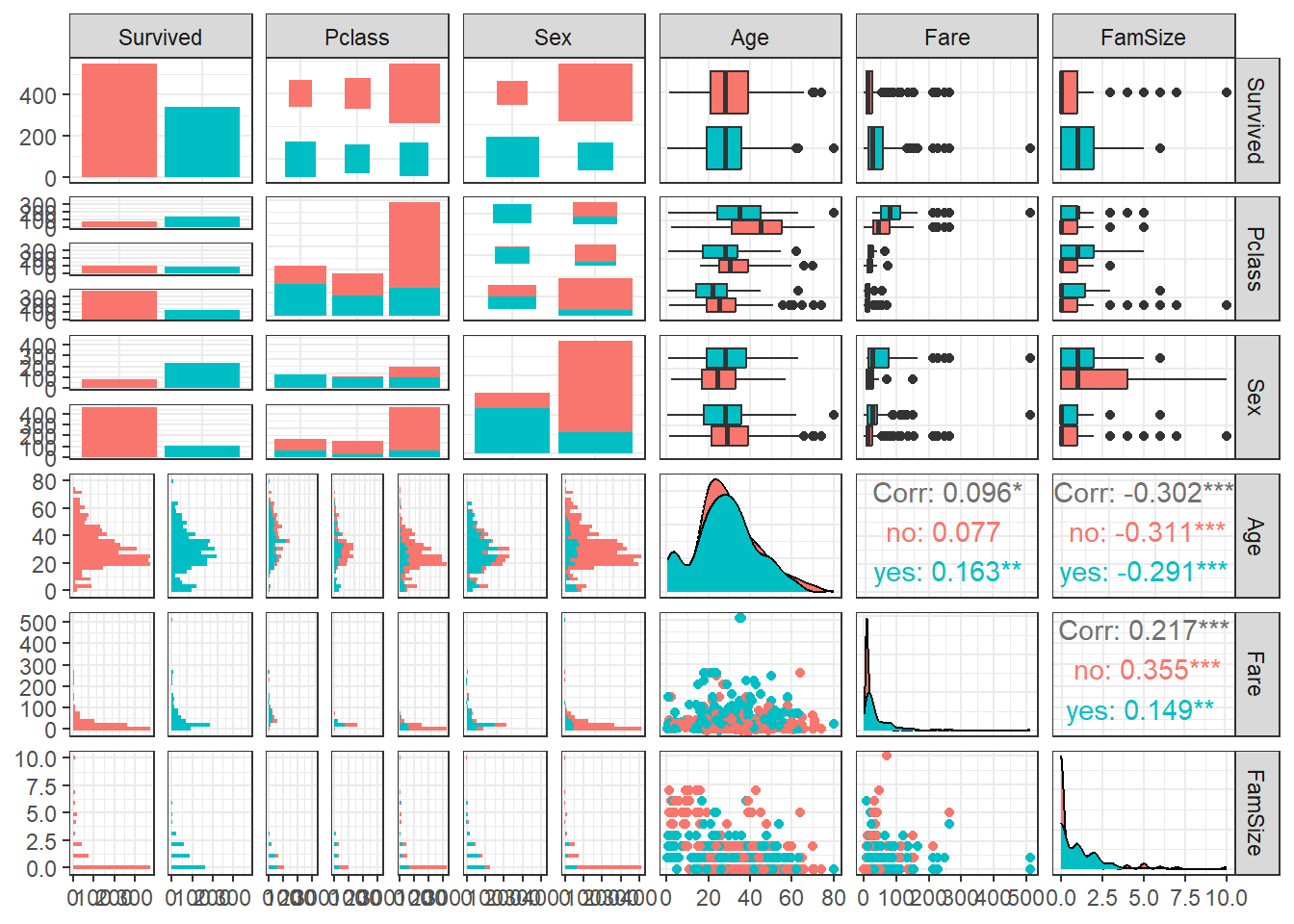
ggpairs(titanic1,
        aes(colour = Survived, alpha = 0.8)) +            # Target의 범주에 따라 색깔을 다르게 표현
  scale_colour_manual(values = c("#00798c", "#d1495b")) + # 특정 색깔 지정
  scale_fill_manual(values = c("#00798c", "#d1495b")) +   # 특정 색깔 지정
  theme_bw()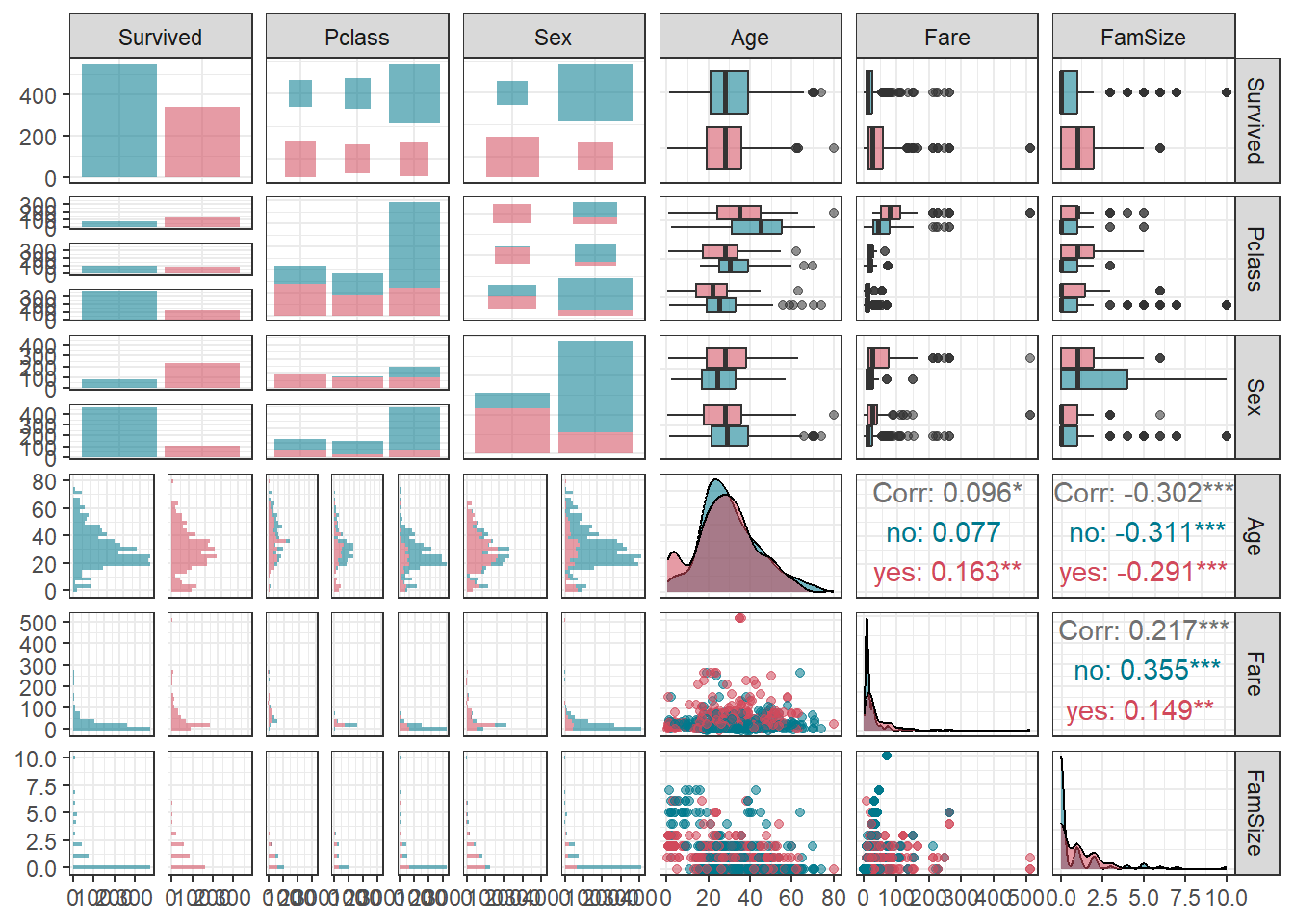
9.4 데이터 분할
# Partition (Training Dataset : Test Dataset = 7:3)
y      <- titanic1$Survived                             # Target

set.seed(200)
ind    <- createDataPartition(y, p = 0.7, list  =T)     # Index를 이용하여 7:3으로 분할
titanic.trd <- titanic1[ind$Resample1,]                 # Training Dataset
titanic.ted <- titanic1[-ind$Resample1,]                # Test Dataset
9.5 데이터 전처리 II
# Imputation
titanic.trd.Imp <- titanic.trd %>%
  mutate(Age = replace_na(Age, mean(Age, na.rm = TRUE)))                 # 평균으로 결측값 대체

titanic.ted.Imp <- titanic.ted %>%
  mutate(Age = replace_na(Age, mean(titanic.trd$Age, na.rm = TRUE)))     # Training Dataset을 이용하여 결측값 대체

glimpse(titanic.trd.Imp)                                                 # 데이터 구조 확인
Rows: 625
Columns: 6
$ Survived <fct> no, yes, yes, no, no, no, yes, yes, yes, yes, no, no, yes, no, yes, no, yes, no, no, no, yes, no, no, yes, yes, no, no, no, no, no, yes, no, no, no, yes, no, yes, no, no, no, yes, n…
$ Pclass <fct> 3, 3, 1, 3, 3, 3, 3, 2, 3, 1, 3, 3, 2, 3, 3, 2, 1, 3, 3, 1, 3, 3, 1, 1, 3, 2, 1, 1, 3, 3, 3, 3, 2, 3, 3, 3, 3, 3, 3, 3, 1, 1, 1, 3, 3, 1, 3, 1, 3, 3, 3, 3, 3, 3, 2, 3, 3, 3, 1, 2, 3…
$ Sex <fct> male, female, female, male, male, male, female, female, female, female, male, female, male, female, female, male, male, female, male, male, female, male, male, female, female, male,…
$ Age <dbl> 22.00000, 26.00000, 35.00000, 35.00000, 29.93737, 2.00000, 27.00000, 14.00000, 4.00000, 58.00000, 39.00000, 14.00000, 29.93737, 31.00000, 29.93737, 35.00000, 28.00000, 8.00000, 29.9…
$ Fare <dbl> 7.2500, 7.9250, 53.1000, 8.0500, 8.4583, 21.0750, 11.1333, 30.0708, 16.7000, 26.5500, 31.2750, 7.8542, 13.0000, 18.0000, 7.2250, 26.0000, 35.5000, 21.0750, 7.2250, 263.0000, 7.8792,…
$ FamSize <int> 1, 0, 1, 0, 0, 4, 2, 1, 2, 0, 6, 0, 0, 1, 0, 0, 0, 4, 0, 5, 0, 0, 0, 1, 0, 0, 1, 1, 0, 2, 1, 1, 1, 0, 0, 1, 0, 2, 1, 5, 1, 1, 0, 7, 0, 0, 5, 0, 2, 7, 1, 0, 0, 0, 2, 0, 0, 0, 0, 0, 3…glimpse(titanic.ted.Imp) # 데이터 구조 확인Rows: 266
Columns: 6
$ Survived <fct> yes, no, no, yes, no, yes, yes, yes, yes, yes, no, no, yes, yes, no, yes, no, yes, yes, no, yes, no, no, no, no, no, no, yes, yes, no, no, no, no, no, no, no, no, no, no, yes, no, n…
$ Pclass <fct> 1, 1, 3, 2, 3, 2, 3, 3, 3, 2, 3, 3, 2, 2, 3, 2, 1, 3, 2, 3, 3, 2, 2, 3, 3, 3, 3, 1, 2, 2, 3, 3, 3, 3, 3, 2, 3, 2, 2, 2, 3, 3, 2, 1, 3, 1, 3, 2, 1, 3, 3, 3, 3, 3, 3, 3, 3, 1, 3, 1, 3…
$ Sex <fct> female, male, male, female, male, male, female, female, male, female, male, male, female, female, male, female, male, male, female, male, female, male, male, male, male, male, male,…
$ Age <dbl> 38.00000, 54.00000, 20.00000, 55.00000, 2.00000, 34.00000, 15.00000, 38.00000, 29.93737, 3.00000, 29.93737, 21.00000, 29.00000, 21.00000, 28.50000, 5.00000, 45.00000, 29.93737, 29.0…
$ Fare <dbl> 71.2833, 51.8625, 8.0500, 16.0000, 29.1250, 13.0000, 8.0292, 31.3875, 7.2292, 41.5792, 8.0500, 7.8000, 26.0000, 10.5000, 7.2292, 27.7500, 83.4750, 15.2458, 10.5000, 8.1583, 7.9250, …
$ FamSize <int> 1, 0, 0, 0, 5, 0, 0, 6, 0, 3, 0, 0, 1, 0, 0, 3, 1, 2, 0, 0, 6, 0, 0, 0, 0, 4, 0, 1, 1, 1, 0, 0, 0, 0, 0, 1, 6, 2, 1, 0, 0, 1, 0, 2, 0, 0, 0, 0, 1, 0, 0, 1, 5, 2, 5, 0, 5, 0, 4, 0, 6…9.6 모형 훈련
Package "caret"은 통합 API를 통해 R로 기계 학습을 실행할 수 있는 매우 실용적인 방법을 제공한다. Package "caret"에서는 초모수의 최적의 조합을 찾는 방법으로 그리드 검색(Grid Search), 랜덤 검색(Random Search), 직접 탐색 범위 설정이 있다. 여기서는 초모수 alpha와 lambda의 최적의 조합값을 찾기 위해 그리드 검색을 수행하였고, 이를 기반으로 직접 탐색 범위를 설정하였다. 아래는 그리드 검색을 수행하였을 때 결과이다.
fitControl <- trainControl(method = "cv", number = 5,                 # 5-Fold Cross Validation (5-Fold CV)
                           allowParallel = TRUE)                      # 병렬 처리


set.seed(200)                                                         # For CV
elast.fit <- train(Survived ~ ., data = titanic.trd.Imp,
                   trControl = fitControl ,
                   method = "glmnet",
                   preProc = c("center", "scale"))                    # Standardization for 예측 변수

elast.fit
glmnet
625 samples
5 predictor
2 classes: 'no', 'yes'
Pre-processing: centered (6), scaled (6)
Resampling: Cross-Validated (5 fold)
Summary of sample sizes: 500, 500, 500, 500, 500
Resampling results across tuning parameters:
alpha lambda Accuracy Kappa
0.10 0.0005015509 0.7840 0.5378757
0.10 0.0050155094 0.7840 0.5351176
0.10 0.0501550942 0.7888 0.5401858
0.55 0.0005015509 0.7840 0.5378757
0.55 0.0050155094 0.7840 0.5344038
0.55 0.0501550942 0.7872 0.5392899
1.00 0.0005015509 0.7840 0.5378757
1.00 0.0050155094 0.7856 0.5359368
1.00 0.0501550942 0.7728 0.5149991
Accuracy was used to select the optimal model using the largest value.
The final values used for the model were alpha = 0.1 and lambda = 0.05015509.plot(elast.fit) # Plot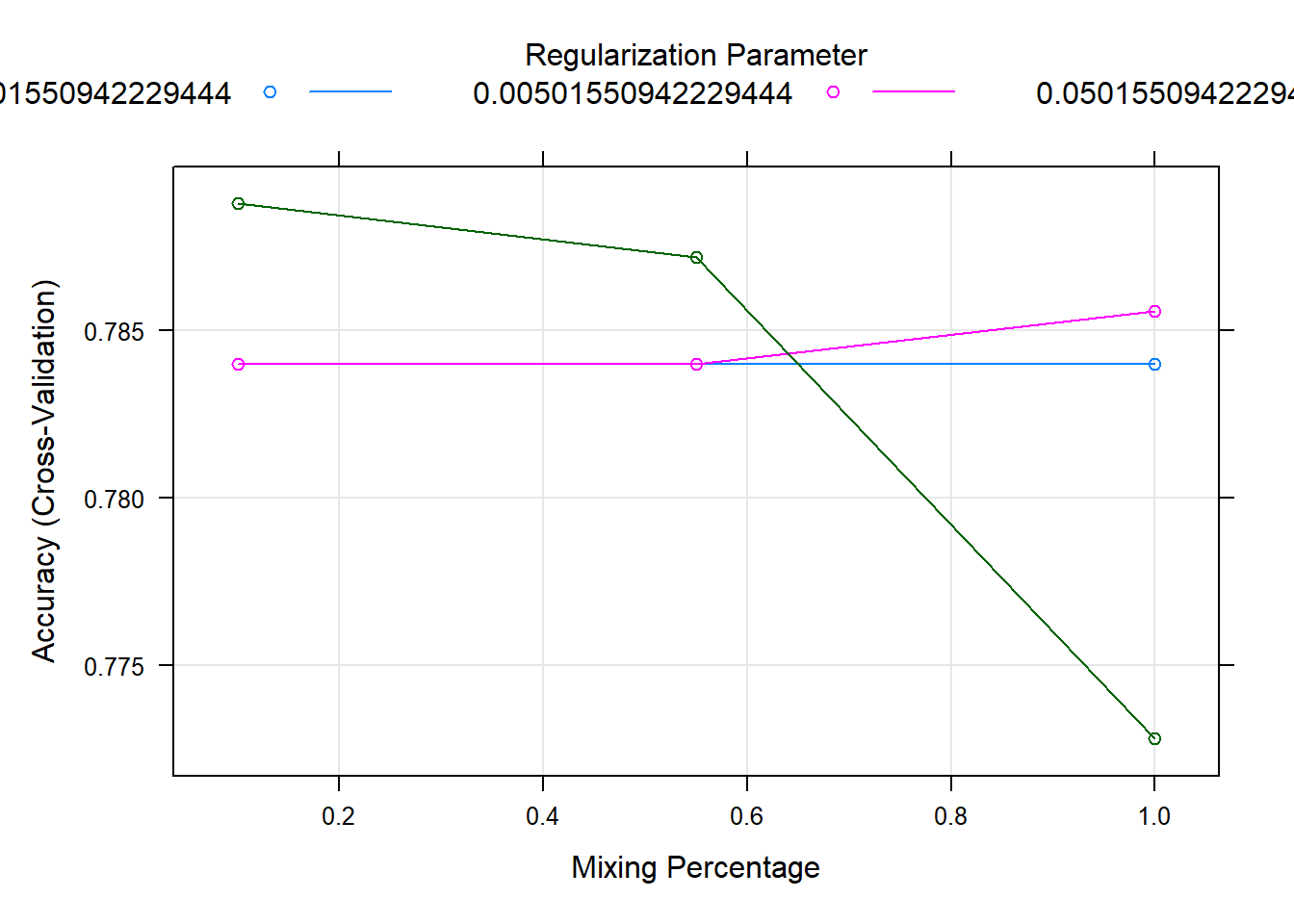
Result! 랜덤하게 결정된 3개의 초모수 alpha, lambda 값을 조합하여 만든 9개의 초모수 조합값 (alpha, lambda)에 대한 정확도를 보여주며, (alpha = 0.1, lambda = 0.05015509)일 때 정확도가 가장 높은 것을 알 수 있다. 따라서 그리드 검색을 통해 찾은 최적의 초모수 조합값 (alpha = 0.1, lambda = 0.05015509) 근처의 값들을 탐색 범위로 설정하여 훈련을 다시 수행할 수 있다.
customGrid <- expand.grid(alpha = seq(0.05, 0.15, by = 0.01),         # alpha의 탐색 범위
                          lambda = seq(0.03, 0.07, by = 0.01))        # lambda의 탐색 범위

set.seed(200)                                                         # For CV
elast.tune.fit <- train(Survived ~ ., data = titanic.trd.Imp,
                        trControl = fitControl ,
                        method = "glmnet",
                        tuneGrid = customGrid,
                        preProc = c("center", "scale"))               # Standardization for 예측 변수

elast.tune.fit
glmnet
625 samples
5 predictor
2 classes: 'no', 'yes'
Pre-processing: centered (6), scaled (6)
Resampling: Cross-Validated (5 fold)
Summary of sample sizes: 500, 500, 500, 500, 500
Resampling results across tuning parameters:
alpha lambda Accuracy Kappa
0.05 0.03 0.7888 0.5408846
0.05 0.04 0.7888 0.5401998
0.05 0.05 0.7888 0.5401998
0.05 0.06 0.7936 0.5463561
0.05 0.07 0.7920 0.5425067
0.06 0.03 0.7888 0.5408846
0.06 0.04 0.7888 0.5401998
0.06 0.05 0.7888 0.5401998
0.06 0.06 0.7936 0.5463561
0.06 0.07 0.7920 0.5425067
0.07 0.03 0.7872 0.5377284
0.07 0.04 0.7888 0.5401998
0.07 0.05 0.7888 0.5401998
0.07 0.06 0.7920 0.5433084
0.07 0.07 0.7920 0.5425067
0.08 0.03 0.7872 0.5377284
0.08 0.04 0.7888 0.5401998
0.08 0.05 0.7888 0.5401998
0.08 0.06 0.7920 0.5433084
0.08 0.07 0.7920 0.5425067
0.09 0.03 0.7856 0.5339514
0.09 0.04 0.7872 0.5370436
0.09 0.05 0.7888 0.5401998
0.09 0.06 0.7920 0.5433084
0.09 0.07 0.7920 0.5425067
0.10 0.03 0.7856 0.5339514
0.10 0.04 0.7872 0.5370436
0.10 0.05 0.7888 0.5401858
0.10 0.06 0.7904 0.5401360
0.10 0.07 0.7904 0.5394590
0.11 0.03 0.7856 0.5339514
0.11 0.04 0.7872 0.5370436
0.11 0.05 0.7888 0.5401858
0.11 0.06 0.7904 0.5401360
0.11 0.07 0.7888 0.5362866
0.12 0.03 0.7856 0.5339514
0.12 0.04 0.7872 0.5370436
0.12 0.05 0.7888 0.5401858
0.12 0.06 0.7904 0.5401360
0.12 0.07 0.7888 0.5362866
0.13 0.03 0.7856 0.5339514
0.13 0.04 0.7872 0.5370436
0.13 0.05 0.7888 0.5401858
0.13 0.06 0.7904 0.5401360
0.13 0.07 0.7888 0.5362866
0.14 0.03 0.7872 0.5377337
0.14 0.04 0.7872 0.5370436
0.14 0.05 0.7888 0.5401858
0.14 0.06 0.7904 0.5401360
0.14 0.07 0.7888 0.5362866
0.15 0.03 0.7872 0.5377337
0.15 0.04 0.7872 0.5370436
0.15 0.05 0.7888 0.5401858
0.15 0.06 0.7920 0.5439542
0.15 0.07 0.7888 0.5362866
Accuracy was used to select the optimal model using the largest value.
The final values used for the model were alpha = 0.05 and lambda = 0.06.plot(elast.tune.fit) # Plot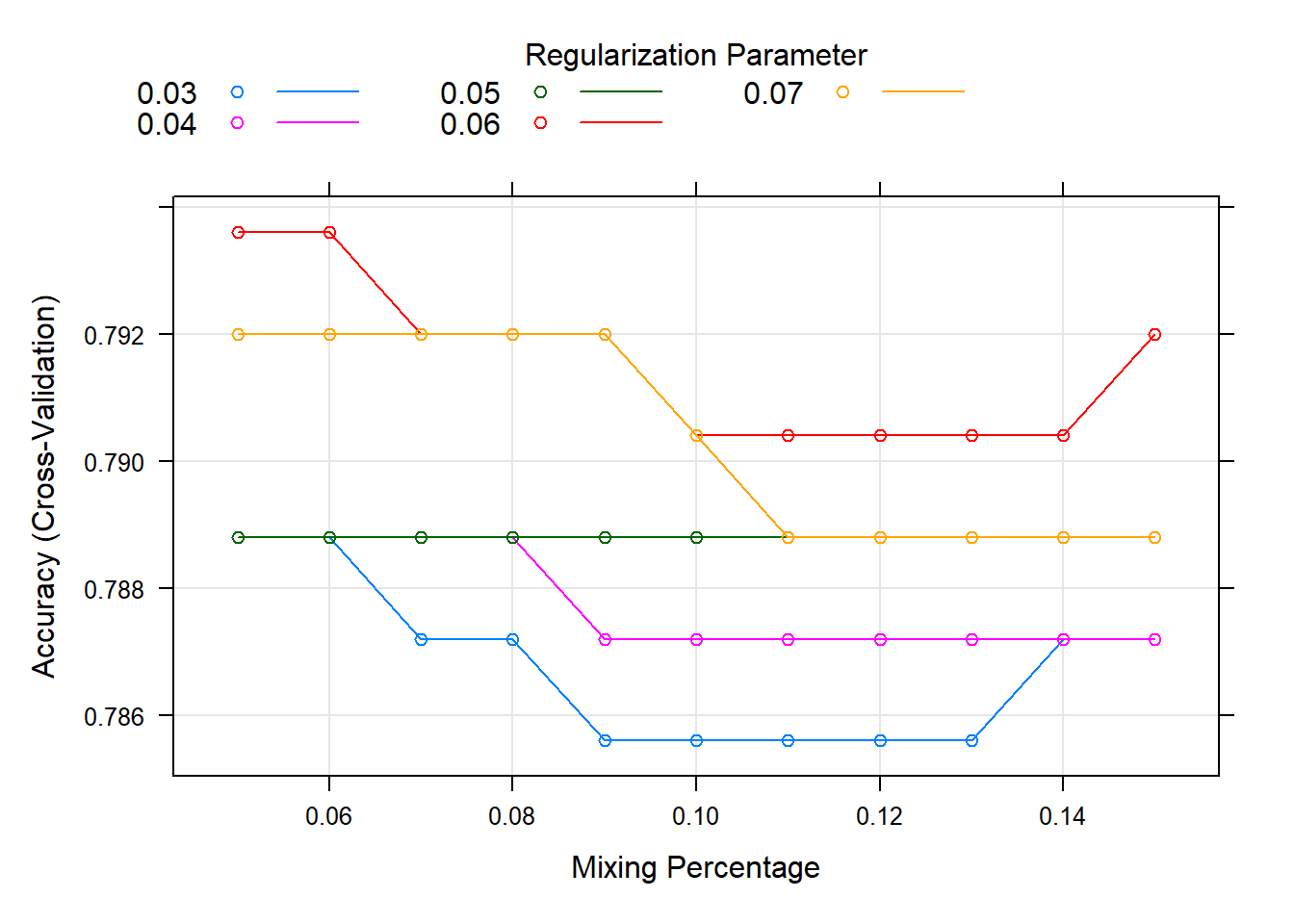
elast.tune.fit$bestTune # 최적의 초모수 조합값 alpha lambda
4 0.05 0.06Result! (alpha = 0.05, lambda = 0.06)일 때 정확도가 가장 높은 것을 알 수 있으며, (alpha = 0.05, lambda = 0.06)를 가지는 모형을 최적의 훈련된 모형으로 선택한다.
round(coef(elast.tune.fit$finalModel, elast.tune.fit$bestTune$lambda), 3) # 최적의 초모수 조합값에 대한 회귀계수 추정치 7 x 1 sparse Matrix of class "dgCMatrix"
s1
(Intercept) -0.565
Pclass2 -0.055
Pclass3 -0.553
Sexmale -0.864
Age -0.233
Fare 0.237
FamSize -0.187Result! 데이터 “titanic.trd.Imp”의 Target “Survived”은 “no”와 “yes” 2개의 클래스를 가지며, “Factor” 변환하면 알파벳순으로 수준을 부여하기 때문에 “yes”가 두 번째 클래스가 된다. 즉, “yes”에 속할 확률(= 탑승객이 생존할 확률)을 \(p\)라고 할 때, 추정된 회귀계수를 이용하여 다음과 같은 모형식을 얻을 수 있다. \[
\begin{align*}
\log{\frac{p}{1-p}} = &-0.565 - 0.055 Z_{\text{Pclass2}} - 0.553 Z_{\text{Pclass3}} -0.864 Z_{\text{Sexmale}} \\
&-0.233 Z_{\text{Age}} +0.237 Z_{\text{Fare}} - 0.187 Z_{\text{FamSize}}
\end{align*}
\] 여기서, \(Z_{\text{예측 변수}}\)는 표준화한 예측 변수를 의미한다.
범주형 예측 변수(“Pclass”, “Sex”)는 더미 변환이 수행되었는데, 예를 들어, Pclass2는 탑승객의 티켓 등급이 2등급인 경우 “1”값을 가지고 2등급이 아니면 “0”값을 가진다.
9.7 모형 평가
Caution! 모형 평가를 위해 Test Dataset에 대한 예측 class/확률 이 필요하며, 함수 predict()를 이용하여 생성한다.
# 예측 class 생성
test.elast.class <- predict(elast.tune.fit,
                            newdata = titanic.ted.Imp[,-1])   # Test Dataset including Only 예측 변수

test.elast.class %>%
  as_tibble
# A tibble: 266 × 1
value
<fct>
1 yes
2 no
3 no
4 yes
5 no
6 no
7 yes
8 no
9 no
10 yes
# ℹ 256 more rows9.7.1 ConfusionMatrix
CM   <- caret::confusionMatrix(test.elast.class, titanic.ted.Imp$Survived,
                               positive = "yes")       # confusionMatrix(예측 class, 실제 class, positive = "관심 class")
CM
Confusion Matrix and Statistics
Reference
Prediction no yes
no 152 36
yes 12 66
Accuracy : 0.8195
95% CI : (0.768, 0.8638)
No Information Rate : 0.6165
P-Value [Acc > NIR] : 5.675e-13
Kappa : 0.6006
Mcnemar's Test P-Value : 0.0009009
Sensitivity : 0.6471
Specificity : 0.9268
Pos Pred Value : 0.8462
Neg Pred Value : 0.8085
Prevalence : 0.3835
Detection Rate : 0.2481
Detection Prevalence : 0.2932
Balanced Accuracy : 0.7869
'Positive' Class : yes
9.7.2 ROC 곡선
# 예측 확률 생성
test.elast.prob <- predict(elast.tune.fit,
                           newdata = titanic.ted.Imp[,-1],# Test Dataset including Only 예측 변수
                           type = "prob")                 # 예측 확률 생성

test.elast.prob %>%
  as_tibble
# A tibble: 266 × 2
no yes
<dbl> <dbl>
1 0.224 0.776
2 0.694 0.306
3 0.821 0.179
4 0.343 0.657
5 0.840 0.160
6 0.686 0.314
7 0.410 0.590
8 0.649 0.351
9 0.846 0.154
10 0.203 0.797
# ℹ 256 more rowstest.elast.prob <- test.elast.prob[,2] # "Survived = yes"에 대한 예측 확률
ac <- titanic.ted.Imp$Survived # Test Dataset의 실제 class
pp <- as.numeric(test.elast.prob) # 예측 확률을 수치형으로 변환9.7.2.1 Package “pROC”
pacman::p_load("pROC")

elast.roc  <- roc(ac, pp, plot = T, col = "gray")      # roc(실제 class, 예측 확률)
auc        <- round(auc(elast.roc), 3)
legend("bottomright", legend = auc, bty = "n")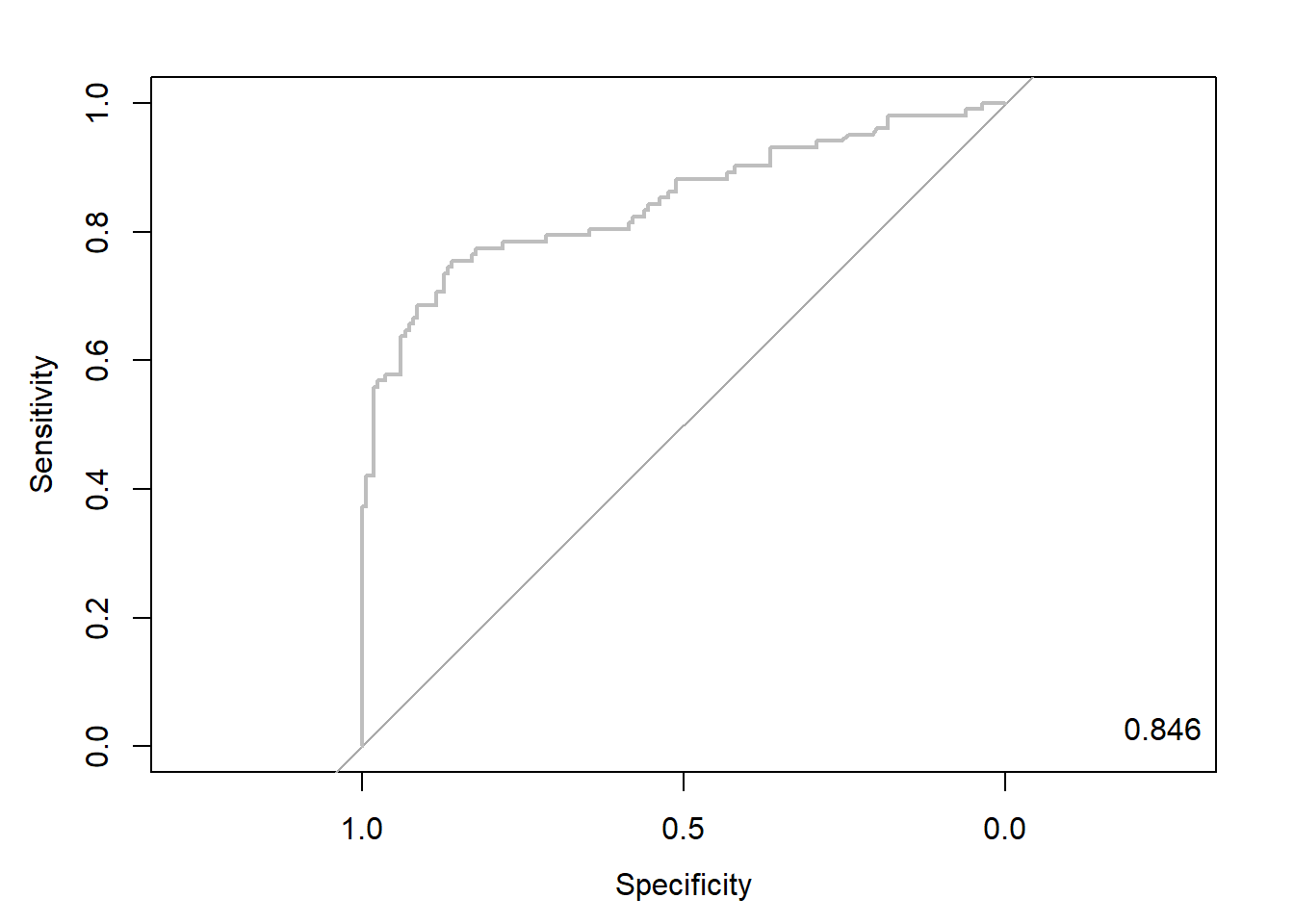
Caution! Package "pROC"를 통해 출력한 ROC 곡선은 다양한 함수를 이용해서 그래프를 수정할 수 있다.
# 함수 plot.roc() 이용
plot.roc(elast.roc,
         col="gray",                                   # Line Color
         print.auc = TRUE,                             # AUC 출력 여부
         print.auc.col = "red",                        # AUC 글씨 색깔
         print.thres = TRUE,                           # Cutoff Value 출력 여부
         print.thres.pch = 19,                         # Cutoff Value를 표시하는 도형 모양
         print.thres.col = "red",                      # Cutoff Value를 표시하는 도형의 색깔
         auc.polygon = TRUE,                           # 곡선 아래 면적에 대한 여부
         auc.polygon.col = "gray90")                   # 곡선 아래 면적의 색깔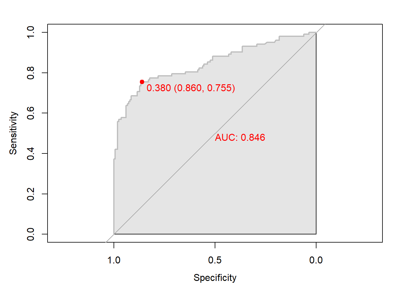
# 함수 ggroc() 이용
ggroc(elast.roc) +
annotate(geom = "text", x = 0.9, y = 1.0,
label = paste("AUC = ", auc),
size = 5,
color="red") +
theme_bw()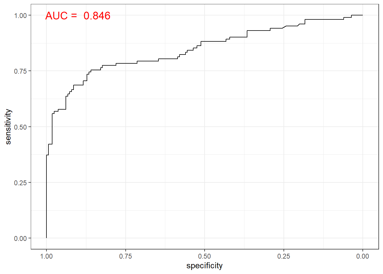
9.7.2.2 Package “Epi”
pacman::p_load("Epi")
# install_version("etm", version = "1.1", repos = "http://cran.us.r-project.org")

ROC(pp, ac, plot = "ROC") # ROC(예측 확률, 실제 class) 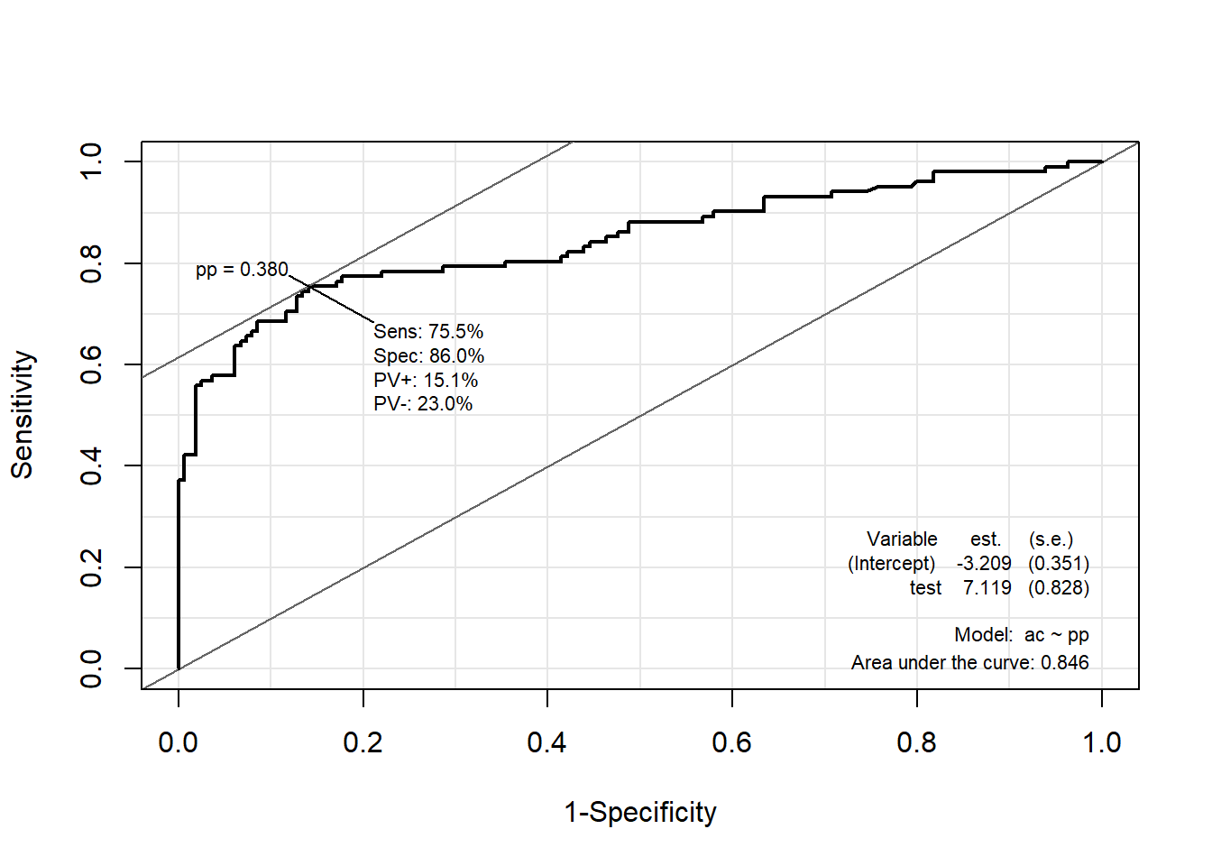
9.7.2.3 Package “ROCR”
pacman::p_load("ROCR")

elast.pred <- prediction(pp, ac)                       # prediction(예측 확률, 실제 class)

elast.perf <- performance(elast.pred, "tpr", "fpr")    # performance(, "민감도", "1-특이도")
plot(elast.perf, col = "gray")                         # ROC Curve

perf.auc   <- performance(elast.pred, "auc")           # AUC
auc        <- attributes(perf.auc)$y.values
legend("bottomright", legend = auc, bty = "n")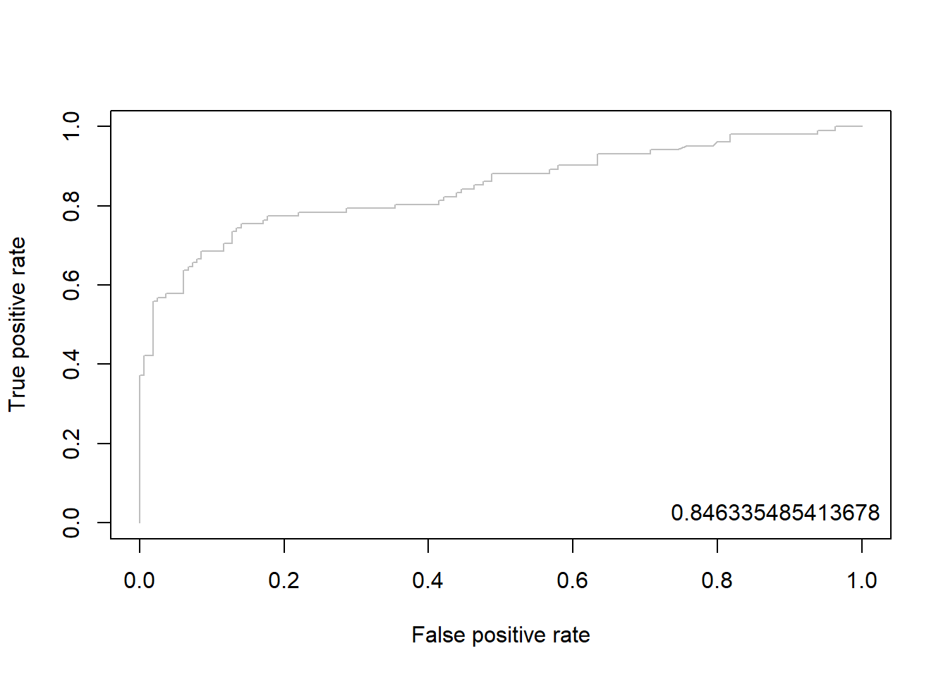
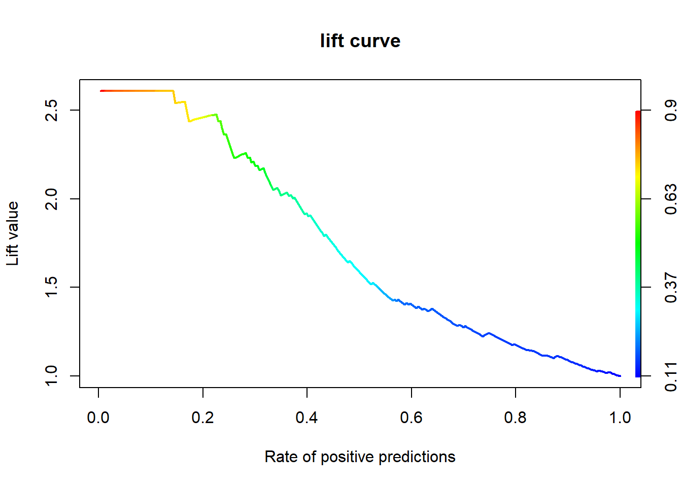
9.7.3 향상 차트
9.7.3.1 Package “ROCR”
elast.perf <- performance(elast.pred, "lift", "rpp")   # Lift Chart
plot(elast.perf, main = "lift curve",
     colorize = T,                                     # Coloring according to cutoff
     lwd = 2)