pacman::p_load("data.table",
               "tidyverse",
               "dplyr", "tidyr",
               "ggplot2", "GGally",
               "caret",
               "doParallel", "parallel")                                # For 병렬 처리

registerDoParallel(cores=detectCores())                                 # 사용할 Core 개수 지정

titanic <- fread("../Titanic.csv")                                      # 데이터 불러오기

titanic %>%
as_tibble8 Ridge Regression
Ridge Regression의 장점
- 규제항을 통해 회귀계수를 “0”에 가깝게 추정한다.
- 회귀계수 추정치의 분산을 감소시켜
Training Dataset의 변화에도 회귀계수 추정치가 크게 변하지 않는다.
- 회귀계수 추정치의 분산을 감소시켜
Ridge Regression의 단점
- \(\lambda = \infty\)가 아닌 한 회귀계수를 정확하게 “0”으로 추정하지 못한다.
- 변수 선택을 수행할 수 없다.
- 예측변수가 많을 경우 해석이 어렵다.
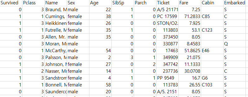
실습 자료 : 1912년 4월 15일 타이타닉호 침몰 당시 탑승객들의 정보를 기록한 데이터셋이며, 총 11개의 변수를 포함하고 있다. 이 자료에서 Target은
Survived이다.

8.1 데이터 불러오기
# A tibble: 891 × 11
   Survived Pclass Name                                                Sex      Age SibSp Parch Ticket            Fare Cabin  Embarked
      <int>  <int> <chr>                                               <chr>  <dbl> <int> <int> <chr>            <dbl> <chr>  <chr>
 1        0      3 Braund, Mr. Owen Harris                             male      22     1     0 A/5 21171         7.25 ""     S
 2        1      1 Cumings, Mrs. John Bradley (Florence Briggs Thayer) female    38     1     0 PC 17599         71.3  "C85"  C
 3        1      3 Heikkinen, Miss. Laina                              female    26     0     0 STON/O2. 3101282  7.92 ""     S
 4        1      1 Futrelle, Mrs. Jacques Heath (Lily May Peel)        female    35     1     0 113803           53.1  "C123" S
 5        0      3 Allen, Mr. William Henry                            male      35     0     0 373450            8.05 ""     S
 6        0      3 Moran, Mr. James                                    male      NA     0     0 330877            8.46 ""     Q
 7        0      1 McCarthy, Mr. Timothy J                             male      54     0     0 17463            51.9  "E46"  S
 8        0      3 Palsson, Master. Gosta Leonard                      male       2     3     1 349909           21.1  ""     S
 9        1      3 Johnson, Mrs. Oscar W (Elisabeth Vilhelmina Berg)   female    27     0     2 347742           11.1  ""     S
10        1      2 Nasser, Mrs. Nicholas (Adele Achem)                 female    14     1     0 237736           30.1  ""     C
# ℹ 881 more rows
8.2 데이터 전처리 I
titanic %<>%
  data.frame() %>%                                                      # Data Frame 형태로 변환
  mutate(Survived = ifelse(Survived == 1, "yes", "no"))                 # Target을 문자형 변수로 변환

# 1. Convert to Factor
fac.col <- c("Pclass", "Sex",
             # Target
             "Survived")

titanic <- titanic %>%
  mutate_at(fac.col, as.factor)                                         # 범주형으로 변환

glimpse(titanic)                                                        # 데이터 구조 확인
Rows: 891
Columns: 11
$ Survived <fct> no, yes, yes, yes, no, no, no, no, yes, yes, yes, yes, no, no, no, yes, no, yes, no, yes, no, yes, yes, yes, no, yes, no, no, yes, no, no, yes, yes, no, no, no, yes, no, no, yes, no…
$ Pclass <fct> 3, 1, 3, 1, 3, 3, 1, 3, 3, 2, 3, 1, 3, 3, 3, 2, 3, 2, 3, 3, 2, 2, 3, 1, 3, 3, 3, 1, 3, 3, 1, 1, 3, 2, 1, 1, 3, 3, 3, 3, 3, 2, 3, 2, 3, 3, 3, 3, 3, 3, 3, 3, 1, 2, 1, 1, 2, 3, 2, 3, 3…
$ Name <chr> "Braund, Mr. Owen Harris", "Cumings, Mrs. John Bradley (Florence Briggs Thayer)", "Heikkinen, Miss. Laina", "Futrelle, Mrs. Jacques Heath (Lily May Peel)", "Allen, Mr. William Henry…
$ Sex <fct> male, female, female, female, male, male, male, male, female, female, female, female, male, male, female, female, male, male, female, female, male, male, female, male, female, femal…
$ Age <dbl> 22.0, 38.0, 26.0, 35.0, 35.0, NA, 54.0, 2.0, 27.0, 14.0, 4.0, 58.0, 20.0, 39.0, 14.0, 55.0, 2.0, NA, 31.0, NA, 35.0, 34.0, 15.0, 28.0, 8.0, 38.0, NA, 19.0, NA, NA, 40.0, NA, NA, 66.…
$ SibSp <int> 1, 1, 0, 1, 0, 0, 0, 3, 0, 1, 1, 0, 0, 1, 0, 0, 4, 0, 1, 0, 0, 0, 0, 0, 3, 1, 0, 3, 0, 0, 0, 1, 0, 0, 1, 1, 0, 0, 2, 1, 1, 1, 0, 1, 0, 0, 1, 0, 2, 1, 4, 0, 1, 1, 0, 0, 0, 0, 1, 5, 0…
$ Parch <int> 0, 0, 0, 0, 0, 0, 0, 1, 2, 0, 1, 0, 0, 5, 0, 0, 1, 0, 0, 0, 0, 0, 0, 0, 1, 5, 0, 2, 0, 0, 0, 0, 0, 0, 0, 0, 0, 0, 0, 0, 0, 0, 0, 2, 0, 0, 0, 0, 0, 0, 1, 0, 0, 0, 1, 0, 0, 0, 2, 2, 0…
$ Ticket <chr> "A/5 21171", "PC 17599", "STON/O2. 3101282", "113803", "373450", "330877", "17463", "349909", "347742", "237736", "PP 9549", "113783", "A/5. 2151", "347082", "350406", "248706", "38…
$ Fare <dbl> 7.2500, 71.2833, 7.9250, 53.1000, 8.0500, 8.4583, 51.8625, 21.0750, 11.1333, 30.0708, 16.7000, 26.5500, 8.0500, 31.2750, 7.8542, 16.0000, 29.1250, 13.0000, 18.0000, 7.2250, 26.0000,…
$ Cabin <chr> "", "C85", "", "C123", "", "", "E46", "", "", "", "G6", "C103", "", "", "", "", "", "", "", "", "", "D56", "", "A6", "", "", "", "C23 C25 C27", "", "", "", "B78", "", "", "", "", ""…
$ Embarked <chr> "S", "C", "S", "S", "S", "Q", "S", "S", "S", "C", "S", "S", "S", "S", "S", "S", "Q", "S", "S", "C", "S", "S", "Q", "S", "S", "S", "C", "S", "Q", "S", "C", "C", "Q", "S", "C", "S", "…# 2. Generate New Variable
titanic <- titanic %>%
mutate(FamSize = SibSp + Parch) # "FamSize = 형제 및 배우자 수 + 부모님 및 자녀 수"로 가족 수를 의미하는 새로운 변수
glimpse(titanic) # 데이터 구조 확인Rows: 891
Columns: 12
$ Survived <fct> no, yes, yes, yes, no, no, no, no, yes, yes, yes, yes, no, no, no, yes, no, yes, no, yes, no, yes, yes, yes, no, yes, no, no, yes, no, no, yes, yes, no, no, no, yes, no, no, yes, no…
$ Pclass <fct> 3, 1, 3, 1, 3, 3, 1, 3, 3, 2, 3, 1, 3, 3, 3, 2, 3, 2, 3, 3, 2, 2, 3, 1, 3, 3, 3, 1, 3, 3, 1, 1, 3, 2, 1, 1, 3, 3, 3, 3, 3, 2, 3, 2, 3, 3, 3, 3, 3, 3, 3, 3, 1, 2, 1, 1, 2, 3, 2, 3, 3…
$ Name <chr> "Braund, Mr. Owen Harris", "Cumings, Mrs. John Bradley (Florence Briggs Thayer)", "Heikkinen, Miss. Laina", "Futrelle, Mrs. Jacques Heath (Lily May Peel)", "Allen, Mr. William Henry…
$ Sex <fct> male, female, female, female, male, male, male, male, female, female, female, female, male, male, female, female, male, male, female, female, male, male, female, male, female, femal…
$ Age <dbl> 22.0, 38.0, 26.0, 35.0, 35.0, NA, 54.0, 2.0, 27.0, 14.0, 4.0, 58.0, 20.0, 39.0, 14.0, 55.0, 2.0, NA, 31.0, NA, 35.0, 34.0, 15.0, 28.0, 8.0, 38.0, NA, 19.0, NA, NA, 40.0, NA, NA, 66.…
$ SibSp <int> 1, 1, 0, 1, 0, 0, 0, 3, 0, 1, 1, 0, 0, 1, 0, 0, 4, 0, 1, 0, 0, 0, 0, 0, 3, 1, 0, 3, 0, 0, 0, 1, 0, 0, 1, 1, 0, 0, 2, 1, 1, 1, 0, 1, 0, 0, 1, 0, 2, 1, 4, 0, 1, 1, 0, 0, 0, 0, 1, 5, 0…
$ Parch <int> 0, 0, 0, 0, 0, 0, 0, 1, 2, 0, 1, 0, 0, 5, 0, 0, 1, 0, 0, 0, 0, 0, 0, 0, 1, 5, 0, 2, 0, 0, 0, 0, 0, 0, 0, 0, 0, 0, 0, 0, 0, 0, 0, 2, 0, 0, 0, 0, 0, 0, 1, 0, 0, 0, 1, 0, 0, 0, 2, 2, 0…
$ Ticket <chr> "A/5 21171", "PC 17599", "STON/O2. 3101282", "113803", "373450", "330877", "17463", "349909", "347742", "237736", "PP 9549", "113783", "A/5. 2151", "347082", "350406", "248706", "38…
$ Fare <dbl> 7.2500, 71.2833, 7.9250, 53.1000, 8.0500, 8.4583, 51.8625, 21.0750, 11.1333, 30.0708, 16.7000, 26.5500, 8.0500, 31.2750, 7.8542, 16.0000, 29.1250, 13.0000, 18.0000, 7.2250, 26.0000,…
$ Cabin <chr> "", "C85", "", "C123", "", "", "E46", "", "", "", "G6", "C103", "", "", "", "", "", "", "", "", "", "D56", "", "A6", "", "", "", "C23 C25 C27", "", "", "", "B78", "", "", "", "", ""…
$ Embarked <chr> "S", "C", "S", "S", "S", "Q", "S", "S", "S", "C", "S", "S", "S", "S", "S", "S", "Q", "S", "S", "C", "S", "S", "Q", "S", "S", "S", "C", "S", "Q", "S", "C", "C", "Q", "S", "C", "S", "…
$ FamSize <int> 1, 1, 0, 1, 0, 0, 0, 4, 2, 1, 2, 0, 0, 6, 0, 0, 5, 0, 1, 0, 0, 0, 0, 0, 4, 6, 0, 5, 0, 0, 0, 1, 0, 0, 1, 1, 0, 0, 2, 1, 1, 1, 0, 3, 0, 0, 1, 0, 2, 1, 5, 0, 1, 1, 1, 0, 0, 0, 3, 7, 0…# 3. Select Variables used for Analysis
titanic1 <- titanic %>%
select(Survived, Pclass, Sex, Age, Fare, FamSize) # 분석에 사용할 변수 선택
titanic1 %>%
as_tibble# A tibble: 891 × 6
Survived Pclass Sex Age Fare FamSize
<fct> <fct> <fct> <dbl> <dbl> <int>
1 no 3 male 22 7.25 1
2 yes 1 female 38 71.3 1
3 yes 3 female 26 7.92 0
4 yes 1 female 35 53.1 1
5 no 3 male 35 8.05 0
6 no 3 male NA 8.46 0
7 no 1 male 54 51.9 0
8 no 3 male 2 21.1 4
9 yes 3 female 27 11.1 2
10 yes 2 female 14 30.1 1
# ℹ 881 more rows8.3 데이터 탐색
ggpairs(titanic1,
        aes(colour = Survived)) +                         # Target의 범주에 따라 색깔을 다르게 표현
  theme_bw()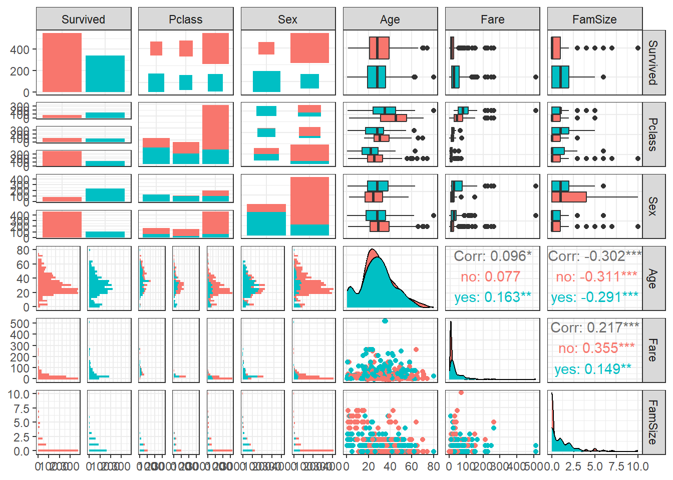
ggpairs(titanic1,
        aes(colour = Survived, alpha = 0.8)) +            # Target의 범주에 따라 색깔을 다르게 표현
  scale_colour_manual(values = c("#00798c", "#d1495b")) + # 특정 색깔 지정
  scale_fill_manual(values = c("#00798c", "#d1495b")) +   # 특정 색깔 지정
  theme_bw()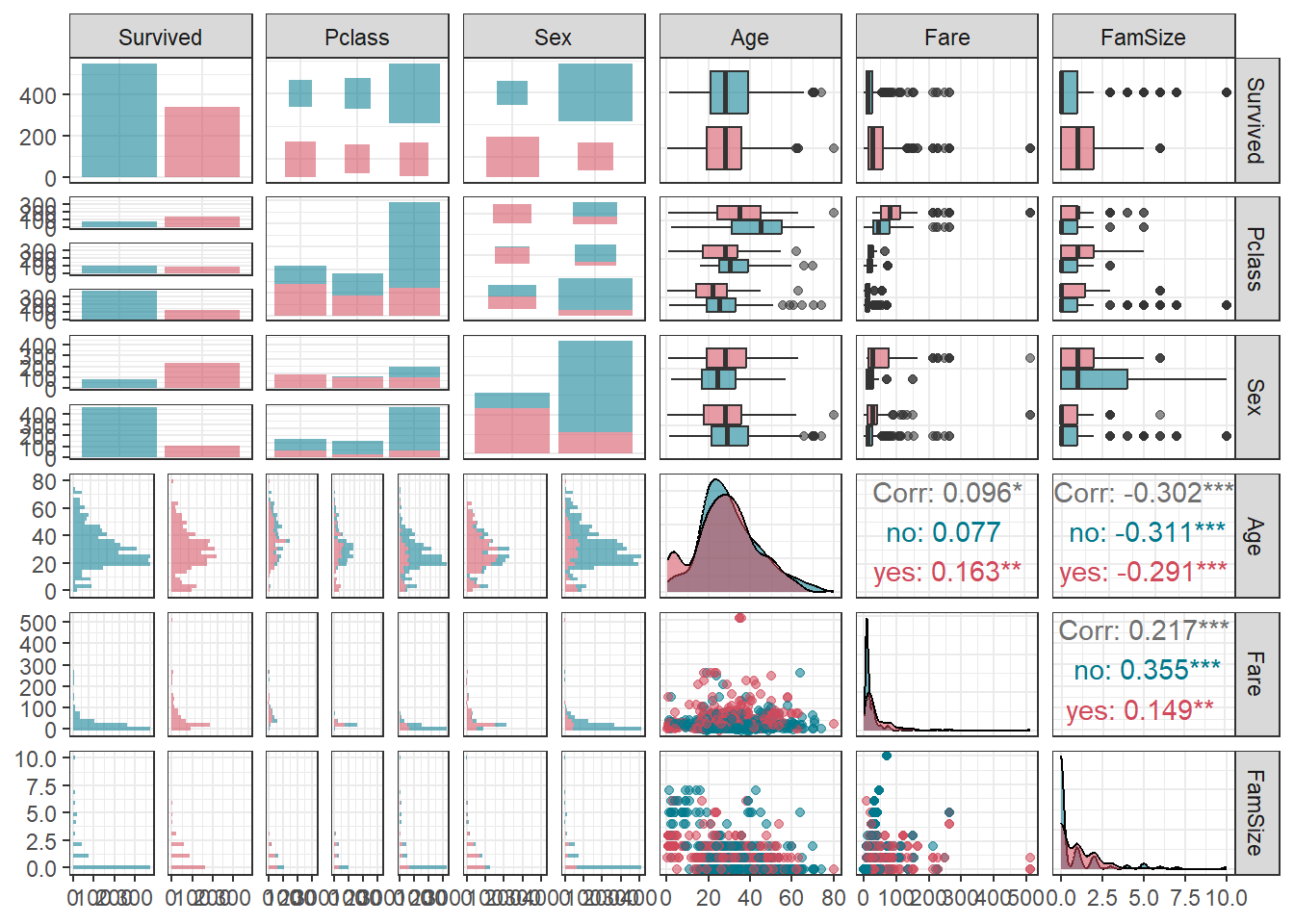
8.4 데이터 분할
# Partition (Training Dataset : Test Dataset = 7:3)
y      <- titanic1$Survived                             # Target

set.seed(200)
ind    <- createDataPartition(y, p = 0.7, list  =T)     # Index를 이용하여 7:3으로 분할
titanic.trd <- titanic1[ind$Resample1,]                 # Training Dataset
titanic.ted <- titanic1[-ind$Resample1,]                # Test Dataset
8.5 데이터 전처리 II
# Imputation
titanic.trd.Imp <- titanic.trd %>%
  mutate(Age = replace_na(Age, mean(Age, na.rm = TRUE)))                 # 평균으로 결측값 대체

titanic.ted.Imp <- titanic.ted %>%
  mutate(Age = replace_na(Age, mean(titanic.trd$Age, na.rm = TRUE)))     # Training Dataset을 이용하여 결측값 대체

glimpse(titanic.trd.Imp)                                                 # 데이터 구조 확인
Rows: 625
Columns: 6
$ Survived <fct> no, yes, yes, no, no, no, yes, yes, yes, yes, no, no, yes, no, yes, no, yes, no, no, no, yes, no, no, yes, yes, no, no, no, no, no, yes, no, no, no, yes, no, yes, no, no, no, yes, n…
$ Pclass <fct> 3, 3, 1, 3, 3, 3, 3, 2, 3, 1, 3, 3, 2, 3, 3, 2, 1, 3, 3, 1, 3, 3, 1, 1, 3, 2, 1, 1, 3, 3, 3, 3, 2, 3, 3, 3, 3, 3, 3, 3, 1, 1, 1, 3, 3, 1, 3, 1, 3, 3, 3, 3, 3, 3, 2, 3, 3, 3, 1, 2, 3…
$ Sex <fct> male, female, female, male, male, male, female, female, female, female, male, female, male, female, female, male, male, female, male, male, female, male, male, female, female, male,…
$ Age <dbl> 22.00000, 26.00000, 35.00000, 35.00000, 29.93737, 2.00000, 27.00000, 14.00000, 4.00000, 58.00000, 39.00000, 14.00000, 29.93737, 31.00000, 29.93737, 35.00000, 28.00000, 8.00000, 29.9…
$ Fare <dbl> 7.2500, 7.9250, 53.1000, 8.0500, 8.4583, 21.0750, 11.1333, 30.0708, 16.7000, 26.5500, 31.2750, 7.8542, 13.0000, 18.0000, 7.2250, 26.0000, 35.5000, 21.0750, 7.2250, 263.0000, 7.8792,…
$ FamSize <int> 1, 0, 1, 0, 0, 4, 2, 1, 2, 0, 6, 0, 0, 1, 0, 0, 0, 4, 0, 5, 0, 0, 0, 1, 0, 0, 1, 1, 0, 2, 1, 1, 1, 0, 0, 1, 0, 2, 1, 5, 1, 1, 0, 7, 0, 0, 5, 0, 2, 7, 1, 0, 0, 0, 2, 0, 0, 0, 0, 0, 3…glimpse(titanic.ted.Imp) # 데이터 구조 확인Rows: 266
Columns: 6
$ Survived <fct> yes, no, no, yes, no, yes, yes, yes, yes, yes, no, no, yes, yes, no, yes, no, yes, yes, no, yes, no, no, no, no, no, no, yes, yes, no, no, no, no, no, no, no, no, no, no, yes, no, n…
$ Pclass <fct> 1, 1, 3, 2, 3, 2, 3, 3, 3, 2, 3, 3, 2, 2, 3, 2, 1, 3, 2, 3, 3, 2, 2, 3, 3, 3, 3, 1, 2, 2, 3, 3, 3, 3, 3, 2, 3, 2, 2, 2, 3, 3, 2, 1, 3, 1, 3, 2, 1, 3, 3, 3, 3, 3, 3, 3, 3, 1, 3, 1, 3…
$ Sex <fct> female, male, male, female, male, male, female, female, male, female, male, male, female, female, male, female, male, male, female, male, female, male, male, male, male, male, male,…
$ Age <dbl> 38.00000, 54.00000, 20.00000, 55.00000, 2.00000, 34.00000, 15.00000, 38.00000, 29.93737, 3.00000, 29.93737, 21.00000, 29.00000, 21.00000, 28.50000, 5.00000, 45.00000, 29.93737, 29.0…
$ Fare <dbl> 71.2833, 51.8625, 8.0500, 16.0000, 29.1250, 13.0000, 8.0292, 31.3875, 7.2292, 41.5792, 8.0500, 7.8000, 26.0000, 10.5000, 7.2292, 27.7500, 83.4750, 15.2458, 10.5000, 8.1583, 7.9250, …
$ FamSize <int> 1, 0, 0, 0, 5, 0, 0, 6, 0, 3, 0, 0, 1, 0, 0, 3, 1, 2, 0, 0, 6, 0, 0, 0, 0, 4, 0, 1, 1, 1, 0, 0, 0, 0, 0, 1, 6, 2, 1, 0, 0, 1, 0, 2, 0, 0, 0, 0, 1, 0, 0, 1, 5, 2, 5, 0, 5, 0, 4, 0, 6…8.6 모형 훈련
Package "caret"은 통합 API를 통해 R로 기계 학습을 실행할 수 있는 매우 실용적인 방법을 제공한다. Package "caret"를 통해 Ridge Regression을 수행하기 위해 옵션 method에 다양한 방법(Ex: "ridge", "foba" 등)을 입력할 수 있지만, 대부분 회귀 문제에 대해서만 분석이 가능하다. 분류와 회귀 문제 모두 가능한 "glmnet"을 이용하려면 옵션 tuneGrid = expand.grid()을 통해 탐색하고자 하는 초모수 lambda의 범위를 직접 지정해줘야 한다.
fitControl <- trainControl(method = "cv", number = 5,                 # 5-Fold Cross Validation (5-Fold CV)
                           allowParallel = TRUE)                      # 병렬 처리

set.seed(200)                                                         # For CV
ridge.fit <- train(Survived ~ ., data = titanic.trd.Imp,
                   trControl = fitControl ,
                   method = "glmnet",
                   tuneGrid = expand.grid(alpha = 0,                  # For Ridge Regression
                                          lambda = seq(0, 1, 0.001)), # lambda의 탐색 범위
                   preProc = c("center", "scale"))                    # Standardization for 예측 변수

ridge.fit
glmnet
625 samples
5 predictor
2 classes: 'no', 'yes'
Pre-processing: centered (6), scaled (6)
Resampling: Cross-Validated (5 fold)
Summary of sample sizes: 500, 500, 500, 500, 500
Resampling results across tuning parameters:
lambda Accuracy Kappa
0.000 0.7920 0.5477147
0.001 0.7920 0.5477147
0.002 0.7920 0.5477147
0.003 0.7920 0.5477147
0.004 0.7920 0.5477147
0.005 0.7920 0.5477147
0.006 0.7920 0.5477147
0.007 0.7920 0.5477147
0.008 0.7920 0.5477147
0.009 0.7920 0.5477147
0.010 0.7920 0.5477147
0.011 0.7920 0.5477147
0.012 0.7920 0.5477147
0.013 0.7920 0.5477147
0.014 0.7920 0.5477147
0.015 0.7920 0.5477147
0.016 0.7920 0.5477147
0.017 0.7920 0.5477147
0.018 0.7920 0.5477147
0.019 0.7920 0.5477147
0.020 0.7920 0.5477147
0.021 0.7920 0.5477147
0.022 0.7920 0.5477147
0.023 0.7920 0.5477147
0.024 0.7920 0.5477147
0.025 0.7920 0.5477147
0.026 0.7920 0.5477147
0.027 0.7904 0.5439323
0.028 0.7904 0.5439323
0.029 0.7904 0.5439323
0.030 0.7904 0.5439323
0.031 0.7888 0.5408846
0.032 0.7888 0.5408846
0.033 0.7904 0.5439795
0.034 0.7904 0.5439795
0.035 0.7904 0.5439795
0.036 0.7904 0.5439795
0.037 0.7904 0.5439795
0.038 0.7904 0.5439795
0.039 0.7888 0.5401998
0.040 0.7888 0.5401998
0.041 0.7888 0.5401998
0.042 0.7888 0.5401998
0.043 0.7888 0.5401998
0.044 0.7888 0.5401998
0.045 0.7888 0.5401998
0.046 0.7904 0.5432476
0.047 0.7904 0.5432476
0.048 0.7904 0.5432476
0.049 0.7936 0.5495496
0.050 0.7952 0.5526223
0.051 0.7952 0.5526223
0.052 0.7952 0.5526223
0.053 0.7984 0.5588816
0.054 0.7984 0.5588816
0.055 0.7968 0.5550660
0.056 0.7968 0.5550660
0.057 0.7968 0.5550660
0.058 0.7984 0.5582310
0.059 0.7984 0.5582310
0.060 0.7952 0.5503013
0.061 0.7952 0.5494856
0.062 0.7952 0.5494856
0.063 0.7952 0.5494856
0.064 0.7952 0.5494856
0.065 0.7952 0.5494856
0.066 0.7952 0.5494856
0.067 0.7952 0.5494856
0.068 0.7936 0.5456362
0.069 0.7936 0.5456362
0.070 0.7936 0.5456362
0.071 0.7920 0.5418538
0.072 0.7920 0.5418538
0.073 0.7904 0.5380410
0.074 0.7904 0.5380410
0.075 0.7920 0.5411832
0.076 0.7920 0.5411832
0.077 0.7920 0.5411832
0.078 0.7920 0.5411832
0.079 0.7920 0.5411832
0.080 0.7920 0.5411832
0.081 0.7920 0.5411832
0.082 0.7904 0.5373676
0.083 0.7904 0.5373676
0.084 0.7904 0.5373676
0.085 0.7904 0.5373676
0.086 0.7920 0.5405558
0.087 0.7920 0.5405558
0.088 0.7920 0.5405558
0.089 0.7920 0.5405558
0.090 0.7920 0.5405558
0.091 0.7920 0.5392003
0.092 0.7936 0.5424629
0.093 0.7920 0.5384109
0.094 0.7920 0.5384109
0.095 0.7920 0.5384109
0.096 0.7920 0.5384109
0.097 0.7920 0.5384109
0.098 0.7920 0.5384109
0.099 0.7904 0.5345671
0.100 0.7904 0.5345671
0.101 0.7920 0.5378571
0.102 0.7920 0.5378571
0.103 0.7936 0.5410796
0.104 0.7936 0.5410796
0.105 0.7936 0.5410796
0.106 0.7936 0.5410796
0.107 0.7936 0.5410796
0.108 0.7936 0.5410796
0.109 0.7936 0.5410796
0.110 0.7904 0.5322904
0.111 0.7920 0.5355403
0.112 0.7904 0.5316909
0.113 0.7904 0.5309466
0.114 0.7888 0.5256137
0.115 0.7888 0.5256137
0.116 0.7904 0.5288914
0.117 0.7904 0.5288914
0.118 0.7904 0.5288914
0.119 0.7904 0.5288914
0.120 0.7904 0.5288914
0.121 0.7904 0.5288914
0.122 0.7904 0.5288914
0.123 0.7904 0.5288914
0.124 0.7904 0.5288914
0.125 0.7888 0.5240297
0.126 0.7872 0.5199325
0.127 0.7872 0.5199325
0.128 0.7872 0.5199325
0.129 0.7856 0.5159047
0.130 0.7856 0.5159047
0.131 0.7856 0.5159047
0.132 0.7856 0.5159047
0.133 0.7824 0.5078909
0.134 0.7824 0.5078909
0.135 0.7824 0.5078909
0.136 0.7792 0.4998192
0.137 0.7808 0.5031216
0.138 0.7808 0.5031216
0.139 0.7808 0.5031216
0.140 0.7808 0.5031216
0.141 0.7808 0.5031216
0.142 0.7808 0.5031216
0.143 0.7792 0.4989892
0.144 0.7792 0.4989892
0.145 0.7792 0.4989892
0.146 0.7792 0.4989892
0.147 0.7792 0.4989892
0.148 0.7792 0.4989892
0.149 0.7792 0.4989892
0.150 0.7792 0.4989892
0.151 0.7792 0.4989892
0.152 0.7792 0.4989892
0.153 0.7792 0.4989892
0.154 0.7792 0.4989892
0.155 0.7792 0.4989892
0.156 0.7776 0.4948531
0.157 0.7776 0.4948531
0.158 0.7760 0.4908685
0.159 0.7760 0.4908685
0.160 0.7760 0.4908685
0.161 0.7760 0.4908685
0.162 0.7760 0.4908685
0.163 0.7760 0.4908685
0.164 0.7760 0.4908685
0.165 0.7760 0.4908685
0.166 0.7744 0.4867002
0.167 0.7712 0.4783236
0.168 0.7712 0.4783236
0.169 0.7728 0.4814732
0.170 0.7744 0.4845893
0.171 0.7744 0.4845893
0.172 0.7744 0.4845893
0.173 0.7744 0.4845893
0.174 0.7744 0.4845893
0.175 0.7744 0.4845893
0.176 0.7744 0.4845893
0.177 0.7744 0.4845893
0.178 0.7744 0.4845893
0.179 0.7744 0.4845893
0.180 0.7744 0.4845893
0.181 0.7744 0.4845893
0.182 0.7728 0.4805782
0.183 0.7728 0.4805782
0.184 0.7728 0.4795092
0.185 0.7728 0.4795092
0.186 0.7728 0.4795092
0.187 0.7744 0.4827385
0.188 0.7760 0.4859375
0.189 0.7760 0.4859375
0.190 0.7760 0.4848850
0.191 0.7760 0.4848850
0.192 0.7760 0.4848850
0.193 0.7760 0.4848850
0.194 0.7760 0.4848850
0.195 0.7760 0.4848850
0.196 0.7744 0.4808102
0.197 0.7728 0.4767011
0.198 0.7728 0.4767011
0.199 0.7728 0.4767011
0.200 0.7728 0.4767011
0.201 0.7728 0.4767011
0.202 0.7712 0.4726796
0.203 0.7712 0.4726796
0.204 0.7712 0.4726796
0.205 0.7712 0.4726796
0.206 0.7728 0.4758139
0.207 0.7728 0.4758139
0.208 0.7728 0.4758139
0.209 0.7728 0.4758139
0.210 0.7728 0.4758139
0.211 0.7728 0.4758139
0.212 0.7728 0.4758139
0.213 0.7728 0.4758139
0.214 0.7728 0.4750117
0.215 0.7728 0.4750117
0.216 0.7728 0.4750117
0.217 0.7728 0.4750117
0.218 0.7744 0.4781725
0.219 0.7744 0.4781725
0.220 0.7760 0.4814224
0.221 0.7760 0.4814224
0.222 0.7760 0.4814224
0.223 0.7760 0.4814224
0.224 0.7760 0.4814224
0.225 0.7760 0.4814224
0.226 0.7744 0.4773635
0.227 0.7744 0.4773635
0.228 0.7760 0.4805512
0.229 0.7760 0.4805512
0.230 0.7760 0.4805512
0.231 0.7760 0.4805512
0.232 0.7760 0.4805512
0.233 0.7776 0.4837662
0.234 0.7776 0.4837662
0.235 0.7776 0.4837662
0.236 0.7776 0.4837662
0.237 0.7776 0.4837662
0.238 0.7776 0.4837662
0.239 0.7776 0.4837662
0.240 0.7776 0.4837662
0.241 0.7776 0.4837662
0.242 0.7760 0.4795577
0.243 0.7760 0.4795577
0.244 0.7760 0.4795577
0.245 0.7760 0.4795577
0.246 0.7760 0.4795577
0.247 0.7760 0.4795577
0.248 0.7776 0.4828354
0.249 0.7776 0.4828354
0.250 0.7776 0.4828354
0.251 0.7776 0.4828354
0.252 0.7776 0.4828354
0.253 0.7776 0.4828354
0.254 0.7776 0.4828354
0.255 0.7776 0.4828354
0.256 0.7776 0.4828354
0.257 0.7776 0.4828354
0.258 0.7776 0.4828354
0.259 0.7776 0.4828354
0.260 0.7776 0.4828354
0.261 0.7776 0.4828354
0.262 0.7776 0.4828354
0.263 0.7776 0.4828354
0.264 0.7776 0.4828354
0.265 0.7776 0.4828354
0.266 0.7792 0.4860780
0.267 0.7792 0.4860780
0.268 0.7760 0.4778483
0.269 0.7760 0.4778483
0.270 0.7760 0.4778483
0.271 0.7760 0.4778483
0.272 0.7760 0.4778483
0.273 0.7760 0.4778483
0.274 0.7760 0.4778483
0.275 0.7760 0.4778483
0.276 0.7760 0.4778483
0.277 0.7760 0.4778483
0.278 0.7760 0.4778483
0.279 0.7760 0.4778483
0.280 0.7744 0.4737547
0.281 0.7744 0.4737547
0.282 0.7744 0.4737547
0.283 0.7744 0.4737547
0.284 0.7744 0.4737547
0.285 0.7744 0.4737547
0.286 0.7744 0.4737547
0.287 0.7744 0.4737547
0.288 0.7744 0.4737547
0.289 0.7744 0.4737547
0.290 0.7744 0.4737547
0.291 0.7744 0.4737547
0.292 0.7744 0.4737547
0.293 0.7744 0.4737547
0.294 0.7744 0.4737547
0.295 0.7744 0.4737547
0.296 0.7744 0.4737547
0.297 0.7744 0.4737547
0.298 0.7744 0.4737547
0.299 0.7744 0.4737547
0.300 0.7744 0.4737547
0.301 0.7744 0.4737547
0.302 0.7744 0.4737547
0.303 0.7744 0.4737547
0.304 0.7744 0.4737547
0.305 0.7744 0.4737547
0.306 0.7744 0.4737547
0.307 0.7744 0.4737547
0.308 0.7744 0.4737547
0.309 0.7744 0.4737547
0.310 0.7744 0.4737547
0.311 0.7728 0.4695864
0.312 0.7728 0.4695864
0.313 0.7728 0.4695864
0.314 0.7728 0.4695864
0.315 0.7728 0.4695864
0.316 0.7728 0.4695864
0.317 0.7728 0.4695864
0.318 0.7728 0.4695864
0.319 0.7728 0.4695864
0.320 0.7728 0.4695864
0.321 0.7712 0.4654220
0.322 0.7712 0.4654220
0.323 0.7712 0.4654220
0.324 0.7712 0.4654220
0.325 0.7712 0.4654220
0.326 0.7712 0.4654220
0.327 0.7712 0.4654220
0.328 0.7712 0.4654220
0.329 0.7712 0.4654220
0.330 0.7712 0.4654220
0.331 0.7712 0.4654220
0.332 0.7712 0.4654220
0.333 0.7712 0.4654220
0.334 0.7712 0.4654220
0.335 0.7712 0.4654220
0.336 0.7712 0.4654220
0.337 0.7712 0.4654220
0.338 0.7712 0.4654220
0.339 0.7712 0.4654220
0.340 0.7712 0.4654220
0.341 0.7712 0.4654220
0.342 0.7712 0.4654220
0.343 0.7712 0.4654220
0.344 0.7712 0.4654220
0.345 0.7712 0.4654220
0.346 0.7712 0.4654220
0.347 0.7712 0.4654220
0.348 0.7712 0.4654220
0.349 0.7712 0.4654220
0.350 0.7712 0.4654220
0.351 0.7728 0.4686887
0.352 0.7728 0.4686887
0.353 0.7728 0.4686887
0.354 0.7728 0.4686887
0.355 0.7728 0.4686887
0.356 0.7728 0.4686887
0.357 0.7728 0.4686887
0.358 0.7728 0.4686887
0.359 0.7728 0.4686887
0.360 0.7728 0.4686887
0.361 0.7728 0.4686887
0.362 0.7728 0.4686887
0.363 0.7728 0.4686887
0.364 0.7728 0.4686887
0.365 0.7728 0.4686887
0.366 0.7728 0.4686887
0.367 0.7728 0.4686887
0.368 0.7728 0.4686887
0.369 0.7728 0.4686887
0.370 0.7728 0.4686887
0.371 0.7728 0.4686887
0.372 0.7728 0.4686887
0.373 0.7728 0.4686887
0.374 0.7728 0.4686887
0.375 0.7728 0.4686887
0.376 0.7728 0.4686887
0.377 0.7728 0.4686887
0.378 0.7728 0.4686887
0.379 0.7728 0.4686887
0.380 0.7728 0.4686887
0.381 0.7728 0.4686887
0.382 0.7728 0.4686887
0.383 0.7728 0.4686887
0.384 0.7728 0.4686887
0.385 0.7728 0.4686887
0.386 0.7728 0.4686887
0.387 0.7728 0.4686887
0.388 0.7728 0.4686887
0.389 0.7728 0.4686887
0.390 0.7728 0.4686887
0.391 0.7728 0.4686887
0.392 0.7728 0.4686887
0.393 0.7728 0.4686887
0.394 0.7728 0.4686887
0.395 0.7728 0.4686887
0.396 0.7728 0.4686887
0.397 0.7728 0.4686887
0.398 0.7728 0.4686887
0.399 0.7728 0.4686887
0.400 0.7728 0.4686887
0.401 0.7728 0.4686887
0.402 0.7728 0.4686887
0.403 0.7728 0.4686887
0.404 0.7728 0.4686887
0.405 0.7728 0.4686887
0.406 0.7728 0.4686887
0.407 0.7728 0.4686887
0.408 0.7728 0.4686887
0.409 0.7728 0.4686887
0.410 0.7728 0.4686887
0.411 0.7728 0.4686887
0.412 0.7728 0.4686887
0.413 0.7728 0.4686887
0.414 0.7728 0.4686887
0.415 0.7728 0.4686887
0.416 0.7728 0.4686887
0.417 0.7728 0.4686887
0.418 0.7728 0.4686887
0.419 0.7728 0.4686887
0.420 0.7728 0.4686887
0.421 0.7728 0.4686887
0.422 0.7728 0.4686887
0.423 0.7728 0.4686887
0.424 0.7728 0.4686887
0.425 0.7728 0.4686887
0.426 0.7728 0.4686887
0.427 0.7728 0.4686887
0.428 0.7728 0.4686887
0.429 0.7728 0.4686887
0.430 0.7728 0.4686887
0.431 0.7728 0.4686887
0.432 0.7728 0.4686887
0.433 0.7728 0.4686887
0.434 0.7728 0.4686887
0.435 0.7728 0.4686887
0.436 0.7728 0.4686887
0.437 0.7728 0.4686887
0.438 0.7728 0.4686887
0.439 0.7728 0.4686887
0.440 0.7728 0.4686887
0.441 0.7728 0.4686887
0.442 0.7728 0.4686887
0.443 0.7728 0.4686887
0.444 0.7728 0.4686887
0.445 0.7728 0.4686887
0.446 0.7728 0.4686887
0.447 0.7728 0.4686887
0.448 0.7728 0.4686887
0.449 0.7728 0.4686887
0.450 0.7728 0.4686887
0.451 0.7728 0.4686887
0.452 0.7728 0.4686887
0.453 0.7728 0.4686887
0.454 0.7728 0.4686887
0.455 0.7728 0.4686887
0.456 0.7728 0.4686887
0.457 0.7728 0.4686887
0.458 0.7728 0.4686887
0.459 0.7728 0.4686887
0.460 0.7728 0.4686887
0.461 0.7728 0.4686887
0.462 0.7728 0.4686887
0.463 0.7728 0.4686887
0.464 0.7728 0.4686887
0.465 0.7728 0.4686887
0.466 0.7712 0.4644432
0.467 0.7712 0.4644432
0.468 0.7712 0.4644432
0.469 0.7712 0.4644432
0.470 0.7712 0.4644432
0.471 0.7712 0.4644432
0.472 0.7712 0.4644432
0.473 0.7712 0.4644432
0.474 0.7712 0.4644432
0.475 0.7712 0.4644432
0.476 0.7712 0.4644432
0.477 0.7712 0.4644432
0.478 0.7712 0.4644432
0.479 0.7712 0.4644432
0.480 0.7712 0.4644432
0.481 0.7712 0.4644432
0.482 0.7712 0.4644432
0.483 0.7712 0.4644432
0.484 0.7712 0.4644432
0.485 0.7712 0.4644432
0.486 0.7712 0.4644432
0.487 0.7712 0.4644432
0.488 0.7712 0.4644432
0.489 0.7712 0.4644432
0.490 0.7712 0.4644432
0.491 0.7712 0.4644432
0.492 0.7712 0.4644432
0.493 0.7712 0.4644432
0.494 0.7712 0.4644432
0.495 0.7712 0.4644432
0.496 0.7712 0.4644432
0.497 0.7712 0.4644432
0.498 0.7712 0.4644432
0.499 0.7712 0.4644432
0.500 0.7712 0.4644432
0.501 0.7712 0.4644432
0.502 0.7712 0.4644432
0.503 0.7712 0.4644432
0.504 0.7712 0.4644432
0.505 0.7712 0.4644432
0.506 0.7712 0.4644432
0.507 0.7712 0.4644432
0.508 0.7712 0.4644432
0.509 0.7728 0.4677383
0.510 0.7728 0.4677383
0.511 0.7728 0.4677383
0.512 0.7728 0.4677383
0.513 0.7728 0.4677383
0.514 0.7728 0.4677383
0.515 0.7728 0.4677383
0.516 0.7728 0.4677383
0.517 0.7728 0.4677383
0.518 0.7744 0.4710334
0.519 0.7744 0.4710334
0.520 0.7744 0.4710334
0.521 0.7744 0.4710334
0.522 0.7744 0.4710334
0.523 0.7744 0.4710334
0.524 0.7744 0.4710334
0.525 0.7744 0.4710334
0.526 0.7744 0.4710334
0.527 0.7744 0.4710334
0.528 0.7744 0.4710334
0.529 0.7744 0.4710334
0.530 0.7744 0.4710334
0.531 0.7744 0.4710334
0.532 0.7744 0.4710334
0.533 0.7744 0.4710334
0.534 0.7744 0.4710334
0.535 0.7744 0.4710334
0.536 0.7744 0.4710334
0.537 0.7744 0.4710334
0.538 0.7744 0.4710334
0.539 0.7744 0.4710334
0.540 0.7744 0.4710334
0.541 0.7744 0.4710334
0.542 0.7744 0.4710334
0.543 0.7744 0.4710334
0.544 0.7744 0.4710334
0.545 0.7744 0.4710334
0.546 0.7744 0.4710334
0.547 0.7744 0.4710334
0.548 0.7744 0.4710334
0.549 0.7744 0.4710334
0.550 0.7744 0.4710334
0.551 0.7744 0.4710334
0.552 0.7744 0.4710334
0.553 0.7744 0.4710334
0.554 0.7728 0.4668249
0.555 0.7728 0.4668249
0.556 0.7728 0.4668249
0.557 0.7728 0.4668249
0.558 0.7728 0.4668249
0.559 0.7728 0.4668249
0.560 0.7728 0.4668249
0.561 0.7728 0.4668249
0.562 0.7728 0.4668249
0.563 0.7744 0.4700991
0.564 0.7744 0.4700991
0.565 0.7744 0.4700991
0.566 0.7744 0.4700991
0.567 0.7744 0.4700991
0.568 0.7744 0.4700991
0.569 0.7744 0.4700991
0.570 0.7728 0.4658906
0.571 0.7728 0.4658906
0.572 0.7728 0.4658906
0.573 0.7728 0.4658906
0.574 0.7728 0.4658906
0.575 0.7728 0.4658906
0.576 0.7728 0.4658906
0.577 0.7728 0.4658906
0.578 0.7728 0.4658906
0.579 0.7728 0.4658906
0.580 0.7728 0.4658906
0.581 0.7728 0.4658906
0.582 0.7728 0.4658906
0.583 0.7728 0.4658906
0.584 0.7728 0.4658906
0.585 0.7728 0.4658906
0.586 0.7728 0.4658906
0.587 0.7728 0.4658906
0.588 0.7728 0.4658906
0.589 0.7728 0.4658906
0.590 0.7728 0.4658906
0.591 0.7728 0.4658906
0.592 0.7728 0.4658906
0.593 0.7728 0.4658906
0.594 0.7728 0.4658906
0.595 0.7728 0.4658906
0.596 0.7728 0.4658906
0.597 0.7728 0.4658906
0.598 0.7728 0.4658906
0.599 0.7728 0.4658906
0.600 0.7728 0.4658906
0.601 0.7728 0.4658906
0.602 0.7728 0.4658906
0.603 0.7728 0.4658906
0.604 0.7728 0.4658906
0.605 0.7712 0.4616452
0.606 0.7712 0.4616452
0.607 0.7712 0.4616452
0.608 0.7712 0.4616452
0.609 0.7712 0.4616452
0.610 0.7712 0.4616452
0.611 0.7712 0.4616452
0.612 0.7712 0.4616452
0.613 0.7712 0.4616452
0.614 0.7712 0.4616452
0.615 0.7712 0.4616452
0.616 0.7712 0.4616452
0.617 0.7712 0.4616452
0.618 0.7712 0.4616452
0.619 0.7712 0.4616452
0.620 0.7712 0.4616452
0.621 0.7712 0.4616452
0.622 0.7712 0.4616452
0.623 0.7712 0.4616452
0.624 0.7696 0.4573997
0.625 0.7712 0.4607022
0.626 0.7712 0.4607022
0.627 0.7712 0.4607022
0.628 0.7712 0.4607022
0.629 0.7712 0.4607022
0.630 0.7712 0.4607022
0.631 0.7712 0.4607022
0.632 0.7712 0.4607022
0.633 0.7712 0.4607022
0.634 0.7712 0.4607022
0.635 0.7712 0.4607022
0.636 0.7712 0.4607022
0.637 0.7712 0.4607022
0.638 0.7712 0.4607022
0.639 0.7712 0.4607022
0.640 0.7712 0.4607022
0.641 0.7712 0.4607022
0.642 0.7696 0.4564193
0.643 0.7696 0.4564193
0.644 0.7696 0.4564193
0.645 0.7696 0.4564193
0.646 0.7696 0.4564193
0.647 0.7696 0.4564193
0.648 0.7696 0.4564193
0.649 0.7696 0.4564193
0.650 0.7696 0.4564193
0.651 0.7696 0.4564193
0.652 0.7696 0.4564193
0.653 0.7696 0.4564193
0.654 0.7696 0.4564193
0.655 0.7696 0.4564193
0.656 0.7696 0.4564193
0.657 0.7696 0.4564193
0.658 0.7696 0.4564193
0.659 0.7696 0.4564193
0.660 0.7696 0.4564193
0.661 0.7696 0.4564193
0.662 0.7680 0.4522832
0.663 0.7680 0.4522832
0.664 0.7680 0.4522832
0.665 0.7680 0.4522832
0.666 0.7680 0.4522832
0.667 0.7680 0.4522832
0.668 0.7680 0.4522832
0.669 0.7680 0.4522832
0.670 0.7680 0.4522832
0.671 0.7680 0.4522832
0.672 0.7680 0.4522832
0.673 0.7680 0.4522832
0.674 0.7680 0.4522832
0.675 0.7680 0.4522832
0.676 0.7680 0.4522832
0.677 0.7680 0.4522832
0.678 0.7680 0.4522832
0.679 0.7680 0.4522832
0.680 0.7680 0.4522832
0.681 0.7680 0.4522832
0.682 0.7680 0.4522832
0.683 0.7680 0.4522832
0.684 0.7680 0.4522832
0.685 0.7680 0.4522832
0.686 0.7680 0.4522832
0.687 0.7680 0.4522832
0.688 0.7680 0.4522832
0.689 0.7680 0.4522832
0.690 0.7664 0.4480004
0.691 0.7664 0.4480004
0.692 0.7664 0.4480004
0.693 0.7648 0.4438283
0.694 0.7648 0.4438283
0.695 0.7648 0.4438283
0.696 0.7648 0.4438283
0.697 0.7648 0.4438283
0.698 0.7648 0.4438283
0.699 0.7632 0.4395075
0.700 0.7632 0.4395075
0.701 0.7632 0.4395075
0.702 0.7632 0.4395075
0.703 0.7632 0.4395075
0.704 0.7616 0.4351483
0.705 0.7616 0.4351483
0.706 0.7616 0.4351483
0.707 0.7616 0.4351483
0.708 0.7600 0.4307502
0.709 0.7600 0.4307502
0.710 0.7600 0.4307502
0.711 0.7600 0.4307502
0.712 0.7584 0.4263125
0.713 0.7584 0.4263125
0.714 0.7584 0.4263125
0.715 0.7584 0.4263125
0.716 0.7584 0.4263125
0.717 0.7584 0.4263125
0.718 0.7584 0.4263125
0.719 0.7568 0.4221040
0.720 0.7568 0.4221040
0.721 0.7568 0.4221040
0.722 0.7568 0.4221040
0.723 0.7568 0.4221040
0.724 0.7568 0.4221040
0.725 0.7568 0.4221040
0.726 0.7568 0.4221040
0.727 0.7568 0.4221040
0.728 0.7568 0.4221040
0.729 0.7552 0.4177832
0.730 0.7552 0.4177832
0.731 0.7568 0.4210756
0.732 0.7568 0.4210756
0.733 0.7568 0.4210756
0.734 0.7568 0.4210756
0.735 0.7568 0.4210756
0.736 0.7568 0.4210756
0.737 0.7568 0.4210756
0.738 0.7568 0.4210756
0.739 0.7568 0.4210756
0.740 0.7568 0.4210756
0.741 0.7568 0.4210756
0.742 0.7568 0.4210756
0.743 0.7568 0.4210756
0.744 0.7568 0.4210756
0.745 0.7568 0.4210756
0.746 0.7568 0.4210756
0.747 0.7552 0.4167164
0.748 0.7552 0.4167164
0.749 0.7552 0.4167164
0.750 0.7552 0.4167164
0.751 0.7536 0.4122335
0.752 0.7536 0.4122335
0.753 0.7536 0.4122335
0.754 0.7536 0.4122335
0.755 0.7520 0.4078353
0.756 0.7520 0.4078353
0.757 0.7520 0.4078353
0.758 0.7520 0.4078353
0.759 0.7520 0.4078353
0.760 0.7520 0.4078353
0.761 0.7488 0.3991522
0.762 0.7488 0.3991522
0.763 0.7488 0.3991522
0.764 0.7472 0.3946285
0.765 0.7472 0.3946285
0.766 0.7456 0.3903123
0.767 0.7440 0.3860294
0.768 0.7440 0.3860294
0.769 0.7440 0.3860294
0.770 0.7440 0.3860294
0.771 0.7440 0.3860294
0.772 0.7408 0.3768573
0.773 0.7408 0.3768573
0.774 0.7392 0.3725366
0.775 0.7392 0.3725366
0.776 0.7392 0.3725366
0.777 0.7392 0.3725366
0.778 0.7376 0.3678871
0.779 0.7376 0.3678871
0.780 0.7376 0.3678871
0.781 0.7376 0.3678871
0.782 0.7376 0.3678871
0.783 0.7360 0.3635279
0.784 0.7360 0.3635279
0.785 0.7360 0.3635279
0.786 0.7360 0.3635279
0.787 0.7360 0.3635279
0.788 0.7360 0.3635279
0.789 0.7360 0.3635279
0.790 0.7344 0.3591735
0.791 0.7344 0.3591735
0.792 0.7344 0.3591735
0.793 0.7344 0.3591735
0.794 0.7344 0.3591735
0.795 0.7344 0.3591735
0.796 0.7328 0.3546959
0.797 0.7328 0.3546959
0.798 0.7344 0.3580118
0.799 0.7344 0.3580118
0.800 0.7328 0.3536136
0.801 0.7328 0.3536136
0.802 0.7312 0.3492205
0.803 0.7312 0.3492205
0.804 0.7312 0.3492205
0.805 0.7312 0.3492205
0.806 0.7312 0.3492205
0.807 0.7312 0.3492205
0.808 0.7312 0.3492205
0.809 0.7312 0.3492205
0.810 0.7296 0.3447829
0.811 0.7296 0.3447829
0.812 0.7296 0.3447829
0.813 0.7280 0.3400903
0.814 0.7280 0.3400903
0.815 0.7280 0.3400903
0.816 0.7280 0.3400903
0.817 0.7264 0.3358032
0.818 0.7264 0.3358032
0.819 0.7264 0.3358032
0.820 0.7264 0.3358032
0.821 0.7264 0.3358032
0.822 0.7264 0.3358032
0.823 0.7248 0.3312850
0.824 0.7248 0.3312850
0.825 0.7248 0.3312850
0.826 0.7232 0.3267258
0.827 0.7232 0.3267258
0.828 0.7232 0.3267258
0.829 0.7232 0.3267258
0.830 0.7232 0.3267258
0.831 0.7216 0.3221249
0.832 0.7216 0.3221249
0.833 0.7216 0.3221249
0.834 0.7216 0.3221249
0.835 0.7216 0.3221249
0.836 0.7216 0.3221249
0.837 0.7216 0.3221249
0.838 0.7216 0.3221249
0.839 0.7216 0.3221249
0.840 0.7216 0.3221249
0.841 0.7216 0.3221249
0.842 0.7216 0.3221249
0.843 0.7184 0.3131291
0.844 0.7184 0.3131291
0.845 0.7184 0.3131291
0.846 0.7184 0.3131291
0.847 0.7152 0.3038337
0.848 0.7152 0.3038337
0.849 0.7136 0.2994013
0.850 0.7120 0.2950760
0.851 0.7120 0.2950760
0.852 0.7120 0.2950760
0.853 0.7120 0.2950760
0.854 0.7120 0.2950760
0.855 0.7120 0.2950760
0.856 0.7120 0.2950760
0.857 0.7120 0.2950760
0.858 0.7104 0.2906038
0.859 0.7104 0.2906038
0.860 0.7104 0.2906038
0.861 0.7104 0.2906038
0.862 0.7104 0.2906038
0.863 0.7088 0.2858233
0.864 0.7088 0.2858233
0.865 0.7088 0.2858233
0.866 0.7072 0.2813109
0.867 0.7072 0.2813109
0.868 0.7072 0.2813109
0.869 0.7072 0.2813109
0.870 0.7072 0.2813109
0.871 0.7072 0.2813109
0.872 0.7072 0.2813109
0.873 0.7072 0.2813109
0.874 0.7072 0.2813109
0.875 0.7072 0.2813109
0.876 0.7072 0.2813109
0.877 0.7072 0.2813109
0.878 0.7056 0.2769470
0.879 0.7056 0.2769470
0.880 0.7056 0.2769470
0.881 0.7056 0.2769470
0.882 0.7056 0.2769470
0.883 0.7056 0.2769470
0.884 0.7040 0.2723038
0.885 0.7040 0.2723038
0.886 0.7040 0.2723038
0.887 0.7040 0.2723038
0.888 0.7040 0.2723038
0.889 0.7040 0.2723038
0.890 0.7040 0.2723038
0.891 0.7040 0.2723038
0.892 0.7040 0.2723038
0.893 0.7056 0.2755557
0.894 0.7072 0.2788371
0.895 0.7040 0.2695861
0.896 0.7040 0.2695861
0.897 0.7040 0.2695861
0.898 0.7024 0.2651830
0.899 0.7024 0.2651830
0.900 0.7024 0.2651830
0.901 0.7024 0.2651830
0.902 0.7024 0.2651830
0.903 0.7024 0.2651830
0.904 0.7024 0.2651830
0.905 0.7008 0.2607403
0.906 0.7008 0.2607403
0.907 0.7008 0.2607403
0.908 0.6992 0.2561394
0.909 0.6992 0.2561394
0.910 0.6976 0.2515324
0.911 0.6976 0.2515324
0.912 0.6976 0.2515324
0.913 0.6976 0.2515324
0.914 0.6960 0.2468030
0.915 0.6960 0.2468030
0.916 0.6960 0.2468030
0.917 0.6960 0.2468030
0.918 0.6960 0.2468030
0.919 0.6960 0.2468030
0.920 0.6960 0.2468030
0.921 0.6960 0.2468030
0.922 0.6944 0.2419776
0.923 0.6944 0.2419776
0.924 0.6944 0.2419776
0.925 0.6944 0.2419776
0.926 0.6944 0.2419776
0.927 0.6944 0.2419776
0.928 0.6928 0.2374946
0.929 0.6912 0.2328515
0.930 0.6896 0.2281656
0.931 0.6896 0.2281656
0.932 0.6896 0.2281656
0.933 0.6896 0.2281656
0.934 0.6896 0.2281656
0.935 0.6896 0.2281656
0.936 0.6896 0.2281656
0.937 0.6896 0.2281656
0.938 0.6896 0.2281656
0.939 0.6896 0.2281656
0.940 0.6896 0.2281656
0.941 0.6880 0.2233922
0.942 0.6880 0.2233922
0.943 0.6880 0.2233922
0.944 0.6880 0.2233922
0.945 0.6880 0.2233922
0.946 0.6880 0.2233922
0.947 0.6880 0.2233922
0.948 0.6864 0.2186628
0.949 0.6864 0.2186628
0.950 0.6848 0.2141391
0.951 0.6848 0.2141391
0.952 0.6832 0.2093211
0.953 0.6832 0.2093211
0.954 0.6832 0.2093211
0.955 0.6832 0.2093211
0.956 0.6832 0.2093211
0.957 0.6832 0.2093211
0.958 0.6832 0.2093211
0.959 0.6832 0.2093211
0.960 0.6832 0.2093211
0.961 0.6832 0.2093211
0.962 0.6832 0.2093211
0.963 0.6832 0.2093211
0.964 0.6816 0.2046716
0.965 0.6816 0.2046716
0.966 0.6816 0.2046716
0.967 0.6816 0.2046716
0.968 0.6816 0.2046716
0.969 0.6816 0.2046716
0.970 0.6816 0.2046716
0.971 0.6816 0.2046716
0.972 0.6816 0.2046716
0.973 0.6800 0.1998983
0.974 0.6784 0.1953332
0.975 0.6784 0.1953332
0.976 0.6768 0.1906406
0.977 0.6768 0.1906406
0.978 0.6768 0.1906406
0.979 0.6768 0.1906406
0.980 0.6768 0.1906406
0.981 0.6768 0.1906406
0.982 0.6768 0.1906406
0.983 0.6768 0.1906406
0.984 0.6768 0.1906406
0.985 0.6752 0.1857774
0.986 0.6752 0.1857774
0.987 0.6752 0.1857774
0.988 0.6752 0.1857774
0.989 0.6752 0.1857774
0.990 0.6752 0.1857774
0.991 0.6720 0.1762612
0.992 0.6720 0.1762612
0.993 0.6720 0.1762612
0.994 0.6720 0.1762612
0.995 0.6720 0.1762612
0.996 0.6720 0.1762612
0.997 0.6720 0.1762612
0.998 0.6704 0.1715250
0.999 0.6688 0.1668755
1.000 0.6688 0.1668755
Tuning parameter 'alpha' was held constant at a value of 0
Accuracy was used to select the optimal model using the largest value.
The final values used for the model were alpha = 0 and lambda = 0.059.plot(ridge.fit) # Plot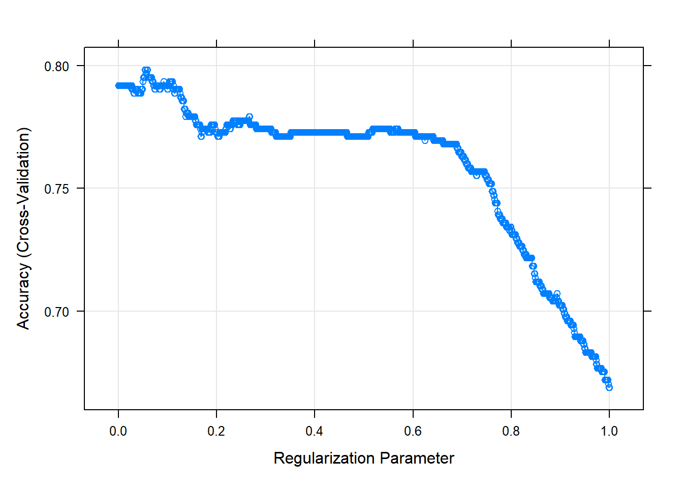
ridge.fit$bestTune # lambda의 최적값 alpha lambda
60 0 0.059Result! lambda = 0.059일 때 정확도가 가장 높은 것을 알 수 있으며, lambda = 0.059를 가지는 모형을 최적의 훈련된 모형으로 선택한다.
round(coef(ridge.fit$finalModel, ridge.fit$bestTune$lambda), 3) # lambda의 최적값에 대한 회귀계수 추정치7 x 1 sparse Matrix of class "dgCMatrix"
s1
(Intercept) -0.566
Pclass2 -0.072
Pclass3 -0.569
Sexmale -0.871
Age -0.251
Fare 0.247
FamSize -0.204Result! 데이터 “titanic.trd.Imp”의 Target “Survived”은 “no”와 “yes” 2개의 클래스를 가지며, “Factor” 변환하면 알파벳순으로 수준을 부여하기 때문에 “yes”가 두 번째 클래스가 된다. 즉, “yes”에 속할 확률(= 탑승객이 생존할 확률)을 \(p\)라고 할 때, 추정된 회귀계수를 이용하여 다음과 같은 모형식을 얻을 수 있다. \[
\begin{align*}
\log{\frac{p}{1-p}} = &-0.566 - 0.072 Z_{\text{Pclass2}} - 0.569 Z_{\text{Pclass3}} -0.871 Z_{\text{Sexmale}} \\
&-0.251 Z_{\text{Age}} +0.247 Z_{\text{Fare}} - 0.204 Z_{\text{FamSize}}
\end{align*}
\] 여기서, \(Z_{\text{예측 변수}}\)는 표준화한 예측 변수를 의미한다.
범주형 예측 변수(“Pclass”, “Sex”)는 더미 변환이 수행되었는데, 예를 들어, Pclass2는 탑승객의 티켓 등급이 2등급인 경우 “1”값을 가지고 2등급이 아니면 “0”값을 가진다.
8.7 모형 평가
Caution! 모형 평가를 위해 Test Dataset에 대한 예측 class/확률 이 필요하며, 함수 predict()를 이용하여 생성한다.
# 예측 class 생성
test.ridge.class <- predict(ridge.fit,
                            newdata = titanic.ted.Imp[,-1]) # Test Dataset including Only 예측 변수

test.ridge.class %>%
  as_tibble
# A tibble: 266 × 1
value
<fct>
1 yes
2 no
3 no
4 yes
5 no
6 no
7 yes
8 no
9 no
10 yes
# ℹ 256 more rows8.7.1 ConfusionMatrix
CM   <- caret::confusionMatrix(test.ridge.class, titanic.ted.Imp$Survived,
                               positive = "yes")       # confusionMatrix(예측 class, 실제 class, positive = "관심 class")
CM
Confusion Matrix and Statistics
Reference
Prediction no yes
no 152 36
yes 12 66
Accuracy : 0.8195
95% CI : (0.768, 0.8638)
No Information Rate : 0.6165
P-Value [Acc > NIR] : 5.675e-13
Kappa : 0.6006
Mcnemar's Test P-Value : 0.0009009
Sensitivity : 0.6471
Specificity : 0.9268
Pos Pred Value : 0.8462
Neg Pred Value : 0.8085
Prevalence : 0.3835
Detection Rate : 0.2481
Detection Prevalence : 0.2932
Balanced Accuracy : 0.7869
'Positive' Class : yes
8.7.2 ROC 곡선
# 예측 확률 생성
test.ridge.prob <- predict(ridge.fit,
                           newdata = titanic.ted.Imp[,-1],# Test Dataset including Only 예측 변수
                           type = "prob")                 # 예측 확률 생성

test.ridge.prob %>%
  as_tibble
# A tibble: 266 × 2
no yes
<dbl> <dbl>
1 0.219 0.781
2 0.694 0.306
3 0.820 0.180
4 0.352 0.648
5 0.842 0.158
6 0.691 0.309
7 0.404 0.596
8 0.663 0.337
9 0.847 0.153
10 0.202 0.798
# ℹ 256 more rowstest.ridge.prob <- test.ridge.prob[,2] # "Survived = yes"에 대한 예측 확률
ac <- titanic.ted.Imp$Survived # Test Dataset의 실제 class
pp <- as.numeric(test.ridge.prob) # 예측 확률을 수치형으로 변환8.7.2.1 Package “pROC”
pacman::p_load("pROC")

ridge.roc  <- roc(ac, pp, plot = T, col = "gray")      # roc(실제 class, 예측 확률)
auc        <- round(auc(ridge.roc), 3)
legend("bottomright", legend = auc, bty = "n")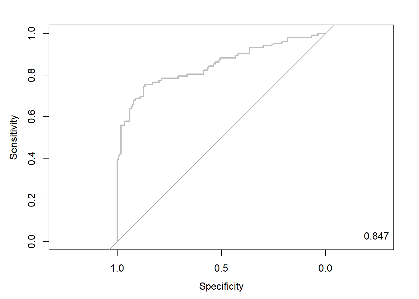
Caution! Package "pROC"를 통해 출력한 ROC 곡선은 다양한 함수를 이용해서 그래프를 수정할 수 있다.
# 함수 plot.roc() 이용
plot.roc(ridge.roc,
         col="gray",                                   # Line Color
         print.auc = TRUE,                             # AUC 출력 여부
         print.auc.col = "red",                        # AUC 글씨 색깔
         print.thres = TRUE,                           # Cutoff Value 출력 여부
         print.thres.pch = 19,                         # Cutoff Value를 표시하는 도형 모양
         print.thres.col = "red",                      # Cutoff Value를 표시하는 도형의 색깔
         auc.polygon = TRUE,                           # 곡선 아래 면적에 대한 여부
         auc.polygon.col = "gray90")                   # 곡선 아래 면적의 색깔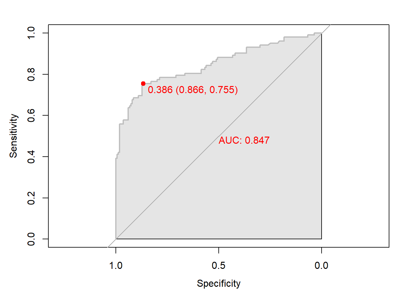
# 함수 ggroc() 이용
ggroc(ridge.roc) +
annotate(geom = "text", x = 0.9, y = 1.0,
label = paste("AUC = ", auc),
size = 5,
color="red") +
theme_bw()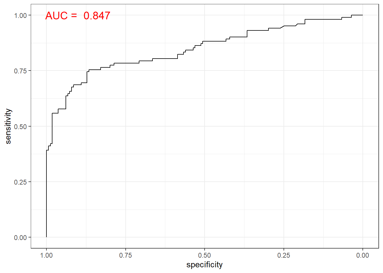
8.7.2.2 Package “Epi”
pacman::p_load("Epi")
# install_version("etm", version = "1.1", repos = "http://cran.us.r-project.org")

ROC(pp, ac, plot = "ROC") # ROC(예측 확률, 실제 class) 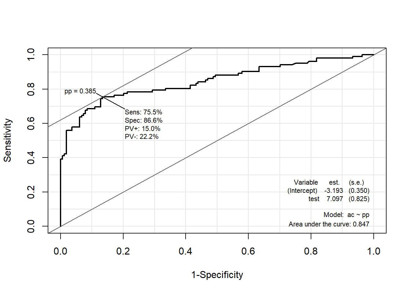
8.7.2.3 Package “ROCR”
pacman::p_load("ROCR")

ridge.pred <- prediction(pp, ac)                       # prediction(예측 확률, 실제 class)

ridge.perf <- performance(ridge.pred, "tpr", "fpr")    # performance(, "민감도", "1-특이도")
plot(ridge.perf, col = "gray")                         # ROC Curve

perf.auc   <- performance(ridge.pred, "auc")           # AUC
auc        <- attributes(perf.auc)$y.values
legend("bottomright", legend = auc, bty = "n")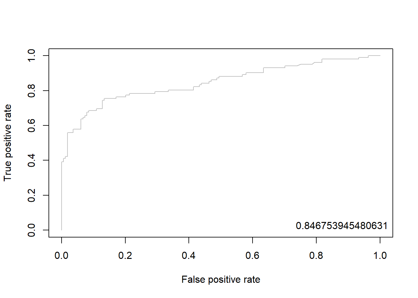
8.7.3 향상 차트
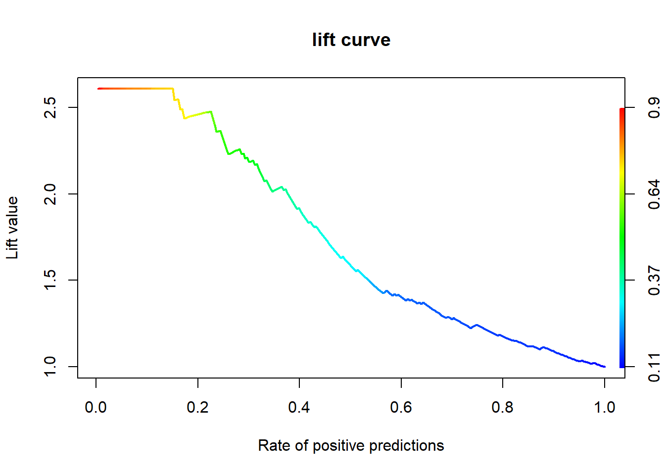
8.7.3.1 Package “ROCR”
ridge.perf <- performance(ridge.pred, "lift", "rpp")   # Lift Chart
plot(ridge.perf, main = "lift curve",
     colorize = T,                                     # Coloring according to cutoff
     lwd = 2)