pacman::p_load("data.table",
               "tidyverse",
               "dplyr", "tidyr",
               "ggplot2", "GGally",
               "caret",
               "doParallel", "parallel")                                # For 병렬 처리

registerDoParallel(cores=detectCores())                                 # 사용할 Core 개수 지정

titanic <- fread("../Titanic.csv")                                      # 데이터 불러오기

titanic %>%
as_tibble5 Support Vector Machine with Polynomial Kernel
Support Vector Machine의 장점
- 분류 경계가 직사각형만 가능한 의사결정나무의 단점을 해결할 수 있다.
- 복잡한 비선형 결정 경계를 학습하는데 유용하다.
- 예측 변수에 분포를 가정하지 않는다.
Support Vector Machine의 단점
- 초모수가 매우 많으며, 초모수에 민감하다.
- 최적의 모형을 찾기 위해 다양한 커널과 초모수의 조합을 평가해야 한다.
- 모형 훈련이 느리다.
- 연속형 예측 변수만 가능하다.
- 범주형 예측 변수는 더미 또는 원-핫 인코딩 변환을 수행해야 한다.
- 해석하기 어려운 복잡한 블랙박스 모형이다.
실습 자료 : 1912년 4월 15일 타이타닉호 침몰 당시 탑승객들의 정보를 기록한 데이터셋이며, 총 11개의 변수를 포함하고 있다. 이 자료에서 Target은
Survived이다.
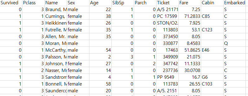

5.1 데이터 불러오기
# A tibble: 891 × 11
   Survived Pclass Name                                                Sex      Age SibSp Parch Ticket            Fare Cabin  Embarked
      <int>  <int> <chr>                                               <chr>  <dbl> <int> <int> <chr>            <dbl> <chr>  <chr>
 1        0      3 Braund, Mr. Owen Harris                             male      22     1     0 A/5 21171         7.25 ""     S
 2        1      1 Cumings, Mrs. John Bradley (Florence Briggs Thayer) female    38     1     0 PC 17599         71.3  "C85"  C
 3        1      3 Heikkinen, Miss. Laina                              female    26     0     0 STON/O2. 3101282  7.92 ""     S
 4        1      1 Futrelle, Mrs. Jacques Heath (Lily May Peel)        female    35     1     0 113803           53.1  "C123" S
 5        0      3 Allen, Mr. William Henry                            male      35     0     0 373450            8.05 ""     S
 6        0      3 Moran, Mr. James                                    male      NA     0     0 330877            8.46 ""     Q
 7        0      1 McCarthy, Mr. Timothy J                             male      54     0     0 17463            51.9  "E46"  S
 8        0      3 Palsson, Master. Gosta Leonard                      male       2     3     1 349909           21.1  ""     S
 9        1      3 Johnson, Mrs. Oscar W (Elisabeth Vilhelmina Berg)   female    27     0     2 347742           11.1  ""     S
10        1      2 Nasser, Mrs. Nicholas (Adele Achem)                 female    14     1     0 237736           30.1  ""     C
# ℹ 881 more rows
5.2 데이터 전처리 I
titanic %<>%
  data.frame() %>%                                                      # Data Frame 형태로 변환
  mutate(Survived = ifelse(Survived == 1, "yes", "no"))                 # Target을 문자형 변수로 변환

# 1. Convert to Factor
fac.col <- c("Pclass", "Sex",
             # Target
             "Survived")

titanic <- titanic %>%
  mutate_at(fac.col, as.factor)                                         # 범주형으로 변환

glimpse(titanic)                                                        # 데이터 구조 확인
Rows: 891
Columns: 11
$ Survived <fct> no, yes, yes, yes, no, no, no, no, yes, yes, yes, yes, no, no, no, yes, no, yes, no, yes, no, yes, yes, yes, no, yes, no, no, yes, no, no, yes, yes, no, no, no, yes, no, no, yes, no…
$ Pclass <fct> 3, 1, 3, 1, 3, 3, 1, 3, 3, 2, 3, 1, 3, 3, 3, 2, 3, 2, 3, 3, 2, 2, 3, 1, 3, 3, 3, 1, 3, 3, 1, 1, 3, 2, 1, 1, 3, 3, 3, 3, 3, 2, 3, 2, 3, 3, 3, 3, 3, 3, 3, 3, 1, 2, 1, 1, 2, 3, 2, 3, 3…
$ Name <chr> "Braund, Mr. Owen Harris", "Cumings, Mrs. John Bradley (Florence Briggs Thayer)", "Heikkinen, Miss. Laina", "Futrelle, Mrs. Jacques Heath (Lily May Peel)", "Allen, Mr. William Henry…
$ Sex <fct> male, female, female, female, male, male, male, male, female, female, female, female, male, male, female, female, male, male, female, female, male, male, female, male, female, femal…
$ Age <dbl> 22.0, 38.0, 26.0, 35.0, 35.0, NA, 54.0, 2.0, 27.0, 14.0, 4.0, 58.0, 20.0, 39.0, 14.0, 55.0, 2.0, NA, 31.0, NA, 35.0, 34.0, 15.0, 28.0, 8.0, 38.0, NA, 19.0, NA, NA, 40.0, NA, NA, 66.…
$ SibSp <int> 1, 1, 0, 1, 0, 0, 0, 3, 0, 1, 1, 0, 0, 1, 0, 0, 4, 0, 1, 0, 0, 0, 0, 0, 3, 1, 0, 3, 0, 0, 0, 1, 0, 0, 1, 1, 0, 0, 2, 1, 1, 1, 0, 1, 0, 0, 1, 0, 2, 1, 4, 0, 1, 1, 0, 0, 0, 0, 1, 5, 0…
$ Parch <int> 0, 0, 0, 0, 0, 0, 0, 1, 2, 0, 1, 0, 0, 5, 0, 0, 1, 0, 0, 0, 0, 0, 0, 0, 1, 5, 0, 2, 0, 0, 0, 0, 0, 0, 0, 0, 0, 0, 0, 0, 0, 0, 0, 2, 0, 0, 0, 0, 0, 0, 1, 0, 0, 0, 1, 0, 0, 0, 2, 2, 0…
$ Ticket <chr> "A/5 21171", "PC 17599", "STON/O2. 3101282", "113803", "373450", "330877", "17463", "349909", "347742", "237736", "PP 9549", "113783", "A/5. 2151", "347082", "350406", "248706", "38…
$ Fare <dbl> 7.2500, 71.2833, 7.9250, 53.1000, 8.0500, 8.4583, 51.8625, 21.0750, 11.1333, 30.0708, 16.7000, 26.5500, 8.0500, 31.2750, 7.8542, 16.0000, 29.1250, 13.0000, 18.0000, 7.2250, 26.0000,…
$ Cabin <chr> "", "C85", "", "C123", "", "", "E46", "", "", "", "G6", "C103", "", "", "", "", "", "", "", "", "", "D56", "", "A6", "", "", "", "C23 C25 C27", "", "", "", "B78", "", "", "", "", ""…
$ Embarked <chr> "S", "C", "S", "S", "S", "Q", "S", "S", "S", "C", "S", "S", "S", "S", "S", "S", "Q", "S", "S", "C", "S", "S", "Q", "S", "S", "S", "C", "S", "Q", "S", "C", "C", "Q", "S", "C", "S", "…# 2. Generate New Variable
titanic <- titanic %>%
mutate(FamSize = SibSp + Parch) # "FamSize = 형제 및 배우자 수 + 부모님 및 자녀 수"로 가족 수를 의미하는 새로운 변수
glimpse(titanic) # 데이터 구조 확인Rows: 891
Columns: 12
$ Survived <fct> no, yes, yes, yes, no, no, no, no, yes, yes, yes, yes, no, no, no, yes, no, yes, no, yes, no, yes, yes, yes, no, yes, no, no, yes, no, no, yes, yes, no, no, no, yes, no, no, yes, no…
$ Pclass <fct> 3, 1, 3, 1, 3, 3, 1, 3, 3, 2, 3, 1, 3, 3, 3, 2, 3, 2, 3, 3, 2, 2, 3, 1, 3, 3, 3, 1, 3, 3, 1, 1, 3, 2, 1, 1, 3, 3, 3, 3, 3, 2, 3, 2, 3, 3, 3, 3, 3, 3, 3, 3, 1, 2, 1, 1, 2, 3, 2, 3, 3…
$ Name <chr> "Braund, Mr. Owen Harris", "Cumings, Mrs. John Bradley (Florence Briggs Thayer)", "Heikkinen, Miss. Laina", "Futrelle, Mrs. Jacques Heath (Lily May Peel)", "Allen, Mr. William Henry…
$ Sex <fct> male, female, female, female, male, male, male, male, female, female, female, female, male, male, female, female, male, male, female, female, male, male, female, male, female, femal…
$ Age <dbl> 22.0, 38.0, 26.0, 35.0, 35.0, NA, 54.0, 2.0, 27.0, 14.0, 4.0, 58.0, 20.0, 39.0, 14.0, 55.0, 2.0, NA, 31.0, NA, 35.0, 34.0, 15.0, 28.0, 8.0, 38.0, NA, 19.0, NA, NA, 40.0, NA, NA, 66.…
$ SibSp <int> 1, 1, 0, 1, 0, 0, 0, 3, 0, 1, 1, 0, 0, 1, 0, 0, 4, 0, 1, 0, 0, 0, 0, 0, 3, 1, 0, 3, 0, 0, 0, 1, 0, 0, 1, 1, 0, 0, 2, 1, 1, 1, 0, 1, 0, 0, 1, 0, 2, 1, 4, 0, 1, 1, 0, 0, 0, 0, 1, 5, 0…
$ Parch <int> 0, 0, 0, 0, 0, 0, 0, 1, 2, 0, 1, 0, 0, 5, 0, 0, 1, 0, 0, 0, 0, 0, 0, 0, 1, 5, 0, 2, 0, 0, 0, 0, 0, 0, 0, 0, 0, 0, 0, 0, 0, 0, 0, 2, 0, 0, 0, 0, 0, 0, 1, 0, 0, 0, 1, 0, 0, 0, 2, 2, 0…
$ Ticket <chr> "A/5 21171", "PC 17599", "STON/O2. 3101282", "113803", "373450", "330877", "17463", "349909", "347742", "237736", "PP 9549", "113783", "A/5. 2151", "347082", "350406", "248706", "38…
$ Fare <dbl> 7.2500, 71.2833, 7.9250, 53.1000, 8.0500, 8.4583, 51.8625, 21.0750, 11.1333, 30.0708, 16.7000, 26.5500, 8.0500, 31.2750, 7.8542, 16.0000, 29.1250, 13.0000, 18.0000, 7.2250, 26.0000,…
$ Cabin <chr> "", "C85", "", "C123", "", "", "E46", "", "", "", "G6", "C103", "", "", "", "", "", "", "", "", "", "D56", "", "A6", "", "", "", "C23 C25 C27", "", "", "", "B78", "", "", "", "", ""…
$ Embarked <chr> "S", "C", "S", "S", "S", "Q", "S", "S", "S", "C", "S", "S", "S", "S", "S", "S", "Q", "S", "S", "C", "S", "S", "Q", "S", "S", "S", "C", "S", "Q", "S", "C", "C", "Q", "S", "C", "S", "…
$ FamSize <int> 1, 1, 0, 1, 0, 0, 0, 4, 2, 1, 2, 0, 0, 6, 0, 0, 5, 0, 1, 0, 0, 0, 0, 0, 4, 6, 0, 5, 0, 0, 0, 1, 0, 0, 1, 1, 0, 0, 2, 1, 1, 1, 0, 3, 0, 0, 1, 0, 2, 1, 5, 0, 1, 1, 1, 0, 0, 0, 3, 7, 0…# 3. Select Variables used for Analysis
titanic1 <- titanic %>%
select(Survived, Pclass, Sex, Age, Fare, FamSize) # 분석에 사용할 변수 선택
# 4. Convert One-hot Encoding for 범주형 예측 변수
dummies <- dummyVars(formula = ~ ., # formula : ~ 예측 변수 / "." : data에 포함된 모든 변수를 의미
data = titanic1[,-1], # Dataset including Only 예측 변수 -> Target 제외
fullRank = FALSE) # fullRank = TRUE : Dummy Variable, fullRank = FALSE : One-hot Encoding
titanic.Var <- predict(dummies, newdata = titanic1) %>% # 범주형 예측 변수에 대한 One-hot Encoding 변환
data.frame() # Data Frame 형태로 변환
glimpse(titanic.Var) # 데이터 구조 확인Rows: 891
Columns: 8
$ Pclass.1 <dbl> 0, 1, 0, 1, 0, 0, 1, 0, 0, 0, 0, 1, 0, 0, 0, 0, 0, 0, 0, 0, 0, 0, 0, 1, 0, 0, 0, 1, 0, 0, 1, 1, 0, 0, 1, 1, 0, 0, 0, 0, 0, 0, 0, 0, 0, 0, 0, 0, 0, 0, 0, 0, 1, 0, 1, 1, 0, 0, 0, 0,…
$ Pclass.2 <dbl> 0, 0, 0, 0, 0, 0, 0, 0, 0, 1, 0, 0, 0, 0, 0, 1, 0, 1, 0, 0, 1, 1, 0, 0, 0, 0, 0, 0, 0, 0, 0, 0, 0, 1, 0, 0, 0, 0, 0, 0, 0, 1, 0, 1, 0, 0, 0, 0, 0, 0, 0, 0, 0, 1, 0, 0, 1, 0, 1, 0,…
$ Pclass.3 <dbl> 1, 0, 1, 0, 1, 1, 0, 1, 1, 0, 1, 0, 1, 1, 1, 0, 1, 0, 1, 1, 0, 0, 1, 0, 1, 1, 1, 0, 1, 1, 0, 0, 1, 0, 0, 0, 1, 1, 1, 1, 1, 0, 1, 0, 1, 1, 1, 1, 1, 1, 1, 1, 0, 0, 0, 0, 0, 1, 0, 1,…
$ Sex.female <dbl> 0, 1, 1, 1, 0, 0, 0, 0, 1, 1, 1, 1, 0, 0, 1, 1, 0, 0, 1, 1, 0, 0, 1, 0, 1, 1, 0, 0, 1, 0, 0, 1, 1, 0, 0, 0, 0, 0, 1, 1, 1, 1, 0, 1, 1, 0, 0, 1, 0, 1, 0, 0, 1, 1, 0, 0, 1, 0, 1, 0,…
$ Sex.male <dbl> 1, 0, 0, 0, 1, 1, 1, 1, 0, 0, 0, 0, 1, 1, 0, 0, 1, 1, 0, 0, 1, 1, 0, 1, 0, 0, 1, 1, 0, 1, 1, 0, 0, 1, 1, 1, 1, 1, 0, 0, 0, 0, 1, 0, 0, 1, 1, 0, 1, 0, 1, 1, 0, 0, 1, 1, 0, 1, 0, 1,…
$ Age <dbl> 22.0, 38.0, 26.0, 35.0, 35.0, NA, 54.0, 2.0, 27.0, 14.0, 4.0, 58.0, 20.0, 39.0, 14.0, 55.0, 2.0, NA, 31.0, NA, 35.0, 34.0, 15.0, 28.0, 8.0, 38.0, NA, 19.0, NA, NA, 40.0, NA, NA, 6…
$ Fare <dbl> 7.2500, 71.2833, 7.9250, 53.1000, 8.0500, 8.4583, 51.8625, 21.0750, 11.1333, 30.0708, 16.7000, 26.5500, 8.0500, 31.2750, 7.8542, 16.0000, 29.1250, 13.0000, 18.0000, 7.2250, 26.000…
$ FamSize <dbl> 1, 1, 0, 1, 0, 0, 0, 4, 2, 1, 2, 0, 0, 6, 0, 0, 5, 0, 1, 0, 0, 0, 0, 0, 4, 6, 0, 5, 0, 0, 0, 1, 0, 0, 1, 1, 0, 0, 2, 1, 1, 1, 0, 3, 0, 0, 1, 0, 2, 1, 5, 0, 1, 1, 1, 0, 0, 0, 3, 7,…# Combine Target with 변환된 예측 변수
titanic.df <- data.frame(Survived = titanic1$Survived,
titanic.Var)
titanic.df %>%
as_tibble# A tibble: 891 × 9
Survived Pclass.1 Pclass.2 Pclass.3 Sex.female Sex.male Age Fare FamSize
<fct> <dbl> <dbl> <dbl> <dbl> <dbl> <dbl> <dbl> <dbl>
1 no 0 0 1 0 1 22 7.25 1
2 yes 1 0 0 1 0 38 71.3 1
3 yes 0 0 1 1 0 26 7.92 0
4 yes 1 0 0 1 0 35 53.1 1
5 no 0 0 1 0 1 35 8.05 0
6 no 0 0 1 0 1 NA 8.46 0
7 no 1 0 0 0 1 54 51.9 0
8 no 0 0 1 0 1 2 21.1 4
9 yes 0 0 1 1 0 27 11.1 2
10 yes 0 1 0 1 0 14 30.1 1
# ℹ 881 more rowsglimpse(titanic.df) # 데이터 구조 확인Rows: 891
Columns: 9
$ Survived <fct> no, yes, yes, yes, no, no, no, no, yes, yes, yes, yes, no, no, no, yes, no, yes, no, yes, no, yes, yes, yes, no, yes, no, no, yes, no, no, yes, yes, no, no, no, yes, no, no, yes, …
$ Pclass.1 <dbl> 0, 1, 0, 1, 0, 0, 1, 0, 0, 0, 0, 1, 0, 0, 0, 0, 0, 0, 0, 0, 0, 0, 0, 1, 0, 0, 0, 1, 0, 0, 1, 1, 0, 0, 1, 1, 0, 0, 0, 0, 0, 0, 0, 0, 0, 0, 0, 0, 0, 0, 0, 0, 1, 0, 1, 1, 0, 0, 0, 0,…
$ Pclass.2 <dbl> 0, 0, 0, 0, 0, 0, 0, 0, 0, 1, 0, 0, 0, 0, 0, 1, 0, 1, 0, 0, 1, 1, 0, 0, 0, 0, 0, 0, 0, 0, 0, 0, 0, 1, 0, 0, 0, 0, 0, 0, 0, 1, 0, 1, 0, 0, 0, 0, 0, 0, 0, 0, 0, 1, 0, 0, 1, 0, 1, 0,…
$ Pclass.3 <dbl> 1, 0, 1, 0, 1, 1, 0, 1, 1, 0, 1, 0, 1, 1, 1, 0, 1, 0, 1, 1, 0, 0, 1, 0, 1, 1, 1, 0, 1, 1, 0, 0, 1, 0, 0, 0, 1, 1, 1, 1, 1, 0, 1, 0, 1, 1, 1, 1, 1, 1, 1, 1, 0, 0, 0, 0, 0, 1, 0, 1,…
$ Sex.female <dbl> 0, 1, 1, 1, 0, 0, 0, 0, 1, 1, 1, 1, 0, 0, 1, 1, 0, 0, 1, 1, 0, 0, 1, 0, 1, 1, 0, 0, 1, 0, 0, 1, 1, 0, 0, 0, 0, 0, 1, 1, 1, 1, 0, 1, 1, 0, 0, 1, 0, 1, 0, 0, 1, 1, 0, 0, 1, 0, 1, 0,…
$ Sex.male <dbl> 1, 0, 0, 0, 1, 1, 1, 1, 0, 0, 0, 0, 1, 1, 0, 0, 1, 1, 0, 0, 1, 1, 0, 1, 0, 0, 1, 1, 0, 1, 1, 0, 0, 1, 1, 1, 1, 1, 0, 0, 0, 0, 1, 0, 0, 1, 1, 0, 1, 0, 1, 1, 0, 0, 1, 1, 0, 1, 0, 1,…
$ Age <dbl> 22.0, 38.0, 26.0, 35.0, 35.0, NA, 54.0, 2.0, 27.0, 14.0, 4.0, 58.0, 20.0, 39.0, 14.0, 55.0, 2.0, NA, 31.0, NA, 35.0, 34.0, 15.0, 28.0, 8.0, 38.0, NA, 19.0, NA, NA, 40.0, NA, NA, 6…
$ Fare <dbl> 7.2500, 71.2833, 7.9250, 53.1000, 8.0500, 8.4583, 51.8625, 21.0750, 11.1333, 30.0708, 16.7000, 26.5500, 8.0500, 31.2750, 7.8542, 16.0000, 29.1250, 13.0000, 18.0000, 7.2250, 26.000…
$ FamSize <dbl> 1, 1, 0, 1, 0, 0, 0, 4, 2, 1, 2, 0, 0, 6, 0, 0, 5, 0, 1, 0, 0, 0, 0, 0, 4, 6, 0, 5, 0, 0, 0, 1, 0, 0, 1, 1, 0, 0, 2, 1, 1, 1, 0, 3, 0, 0, 1, 0, 2, 1, 5, 0, 1, 1, 1, 0, 0, 0, 3, 7,…5.3 데이터 탐색
ggpairs(titanic.df,
        aes(colour = Survived)) +                         # Target의 범주에 따라 색깔을 다르게 표현
  theme_bw()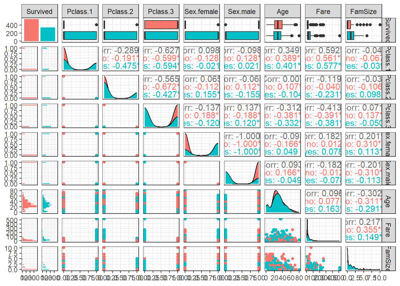
ggpairs(titanic.df,
        aes(colour = Survived, alpha = 0.8)) +            # Target의 범주에 따라 색깔을 다르게 표현
  scale_colour_manual(values = c("#00798c", "#d1495b")) + # 특정 색깔 지정
  scale_fill_manual(values = c("#00798c", "#d1495b")) +   # 특정 색깔 지정
  theme_bw()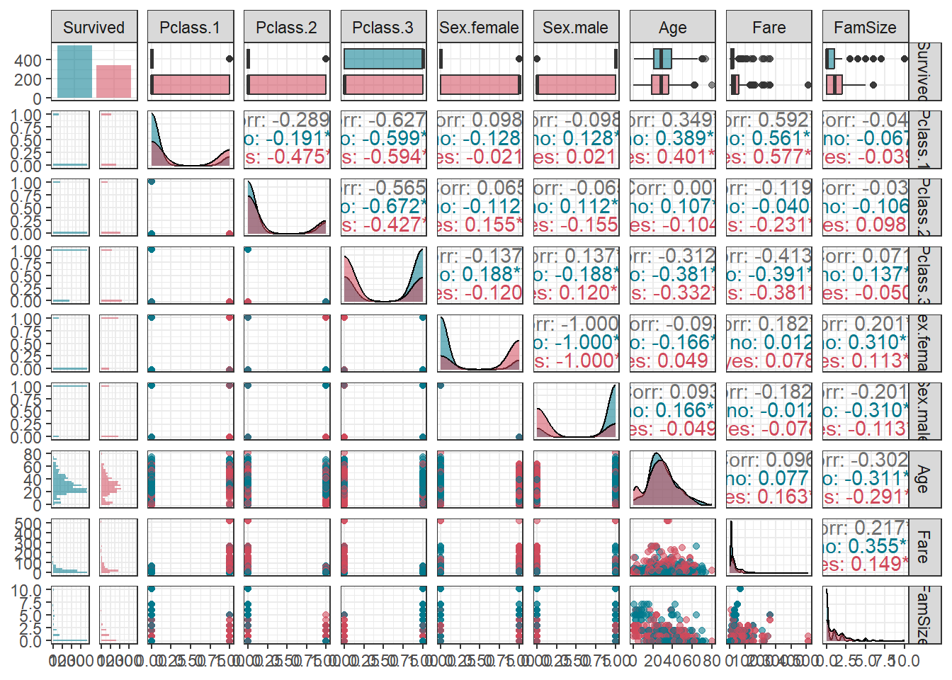
5.4 데이터 분할
# Partition (Training Dataset : Test Dataset = 7:3)
y      <- titanic.df$Survived                           # Target

set.seed(200)
ind    <- createDataPartition(y, p = 0.7, list  =T)     # Index를 이용하여 7:3으로 분할
titanic.trd <- titanic.df[ind$Resample1,]               # Training Dataset
titanic.ted <- titanic.df[-ind$Resample1,]              # Test Dataset
5.5 데이터 전처리 II
# Imputation
titanic.trd.Imp <- titanic.trd %>%
  mutate(Age = replace_na(Age, mean(Age, na.rm = TRUE)))                 # 평균으로 결측값 대체

titanic.ted.Imp <- titanic.ted %>%
  mutate(Age = replace_na(Age, mean(titanic.trd$Age, na.rm = TRUE)))     # Training Dataset을 이용하여 결측값 대체

glimpse(titanic.trd.Imp)                                                 # 데이터 구조 확인
Rows: 625
Columns: 9
$ Survived <fct> no, yes, yes, no, no, no, yes, yes, yes, yes, no, no, yes, no, yes, no, yes, no, no, no, yes, no, no, yes, yes, no, no, no, no, no, yes, no, no, no, yes, no, yes, no, no, no, yes,…
$ Pclass.1 <dbl> 0, 0, 1, 0, 0, 0, 0, 0, 0, 1, 0, 0, 0, 0, 0, 0, 1, 0, 0, 1, 0, 0, 1, 1, 0, 0, 1, 1, 0, 0, 0, 0, 0, 0, 0, 0, 0, 0, 0, 0, 1, 1, 1, 0, 0, 1, 0, 1, 0, 0, 0, 0, 0, 0, 0, 0, 0, 0, 1, 0,…
$ Pclass.2 <dbl> 0, 0, 0, 0, 0, 0, 0, 1, 0, 0, 0, 0, 1, 0, 0, 1, 0, 0, 0, 0, 0, 0, 0, 0, 0, 1, 0, 0, 0, 0, 0, 0, 1, 0, 0, 0, 0, 0, 0, 0, 0, 0, 0, 0, 0, 0, 0, 0, 0, 0, 0, 0, 0, 0, 1, 0, 0, 0, 0, 1,…
$ Pclass.3 <dbl> 1, 1, 0, 1, 1, 1, 1, 0, 1, 0, 1, 1, 0, 1, 1, 0, 0, 1, 1, 0, 1, 1, 0, 0, 1, 0, 0, 0, 1, 1, 1, 1, 0, 1, 1, 1, 1, 1, 1, 1, 0, 0, 0, 1, 1, 0, 1, 0, 1, 1, 1, 1, 1, 1, 0, 1, 1, 1, 0, 0,…
$ Sex.female <dbl> 0, 1, 1, 0, 0, 0, 1, 1, 1, 1, 0, 1, 0, 1, 1, 0, 0, 1, 0, 0, 1, 0, 0, 1, 1, 0, 0, 0, 0, 1, 1, 1, 1, 0, 1, 0, 1, 0, 1, 0, 1, 0, 0, 0, 0, 1, 0, 0, 0, 1, 0, 0, 0, 0, 0, 1, 0, 1, 0, 1,…
$ Sex.male <dbl> 1, 0, 0, 1, 1, 1, 0, 0, 0, 0, 1, 0, 1, 0, 0, 1, 1, 0, 1, 1, 0, 1, 1, 0, 0, 1, 1, 1, 1, 0, 0, 0, 0, 1, 0, 1, 0, 1, 0, 1, 0, 1, 1, 1, 1, 0, 1, 1, 1, 0, 1, 1, 1, 1, 1, 0, 1, 0, 1, 0,…
$ Age <dbl> 22.00000, 26.00000, 35.00000, 35.00000, 29.93737, 2.00000, 27.00000, 14.00000, 4.00000, 58.00000, 39.00000, 14.00000, 29.93737, 31.00000, 29.93737, 35.00000, 28.00000, 8.00000, 29…
$ Fare <dbl> 7.2500, 7.9250, 53.1000, 8.0500, 8.4583, 21.0750, 11.1333, 30.0708, 16.7000, 26.5500, 31.2750, 7.8542, 13.0000, 18.0000, 7.2250, 26.0000, 35.5000, 21.0750, 7.2250, 263.0000, 7.879…
$ FamSize <dbl> 1, 0, 1, 0, 0, 4, 2, 1, 2, 0, 6, 0, 0, 1, 0, 0, 0, 4, 0, 5, 0, 0, 0, 1, 0, 0, 1, 1, 0, 2, 1, 1, 1, 0, 0, 1, 0, 2, 1, 5, 1, 1, 0, 7, 0, 0, 5, 0, 2, 7, 1, 0, 0, 0, 2, 0, 0, 0, 0, 0,…glimpse(titanic.ted.Imp) # 데이터 구조 확인Rows: 266
Columns: 9
$ Survived <fct> yes, no, no, yes, no, yes, yes, yes, yes, yes, no, no, yes, yes, no, yes, no, yes, yes, no, yes, no, no, no, no, no, no, yes, yes, no, no, no, no, no, no, no, no, no, no, yes, no,…
$ Pclass.1 <dbl> 1, 1, 0, 0, 0, 0, 0, 0, 0, 0, 0, 0, 0, 0, 0, 0, 1, 0, 0, 0, 0, 0, 0, 0, 0, 0, 0, 1, 0, 0, 0, 0, 0, 0, 0, 0, 0, 0, 0, 0, 0, 0, 0, 1, 0, 1, 0, 0, 1, 0, 0, 0, 0, 0, 0, 0, 0, 1, 0, 1,…
$ Pclass.2 <dbl> 0, 0, 0, 1, 0, 1, 0, 0, 0, 1, 0, 0, 1, 1, 0, 1, 0, 0, 1, 0, 0, 1, 1, 0, 0, 0, 0, 0, 1, 1, 0, 0, 0, 0, 0, 1, 0, 1, 1, 1, 0, 0, 1, 0, 0, 0, 0, 1, 0, 0, 0, 0, 0, 0, 0, 0, 0, 0, 0, 0,…
$ Pclass.3 <dbl> 0, 0, 1, 0, 1, 0, 1, 1, 1, 0, 1, 1, 0, 0, 1, 0, 0, 1, 0, 1, 1, 0, 0, 1, 1, 1, 1, 0, 0, 0, 1, 1, 1, 1, 1, 0, 1, 0, 0, 0, 1, 1, 0, 0, 1, 0, 1, 0, 0, 1, 1, 1, 1, 1, 1, 1, 1, 0, 1, 0,…
$ Sex.female <dbl> 1, 0, 0, 1, 0, 0, 1, 1, 0, 1, 0, 0, 1, 1, 0, 1, 0, 0, 1, 0, 1, 0, 0, 0, 0, 0, 0, 0, 1, 0, 1, 0, 0, 0, 0, 0, 1, 0, 0, 1, 0, 1, 0, 1, 0, 0, 0, 0, 1, 0, 0, 0, 0, 0, 1, 0, 0, 0, 0, 1,…
$ Sex.male <dbl> 0, 1, 1, 0, 1, 1, 0, 0, 1, 0, 1, 1, 0, 0, 1, 0, 1, 1, 0, 1, 0, 1, 1, 1, 1, 1, 1, 1, 0, 1, 0, 1, 1, 1, 1, 1, 0, 1, 1, 0, 1, 0, 1, 0, 1, 1, 1, 1, 0, 1, 1, 1, 1, 1, 0, 1, 1, 1, 1, 0,…
$ Age <dbl> 38.00000, 54.00000, 20.00000, 55.00000, 2.00000, 34.00000, 15.00000, 38.00000, 29.93737, 3.00000, 29.93737, 21.00000, 29.00000, 21.00000, 28.50000, 5.00000, 45.00000, 29.93737, 29…
$ Fare <dbl> 71.2833, 51.8625, 8.0500, 16.0000, 29.1250, 13.0000, 8.0292, 31.3875, 7.2292, 41.5792, 8.0500, 7.8000, 26.0000, 10.5000, 7.2292, 27.7500, 83.4750, 15.2458, 10.5000, 8.1583, 7.9250…
$ FamSize <dbl> 1, 0, 0, 0, 5, 0, 0, 6, 0, 3, 0, 0, 1, 0, 0, 3, 1, 2, 0, 0, 6, 0, 0, 0, 0, 4, 0, 1, 1, 1, 0, 0, 0, 0, 0, 1, 6, 2, 1, 0, 0, 1, 0, 2, 0, 0, 0, 0, 1, 0, 0, 1, 5, 2, 5, 0, 5, 0, 4, 0,…5.6 모형 훈련
Package "caret"은 통합 API를 통해 R로 기계 학습을 실행할 수 있는 매우 실용적인 방법을 제공한다. Package "caret"에서는 초모수의 최적의 조합을 찾는 방법으로 그리드 검색(Grid Search), 랜덤 검색(Random Search), 직접 탐색 범위 설정이 있다. 여기서는 초모수 degree, scale, C (Cost)의 최적의 조합값을 찾기 위해 그리드 검색을 수행하였고, 이를 기반으로 직접 탐색 범위를 설정하였다. 아래는 그리드 검색을 수행하였을 때 결과이다.
fitControl <- trainControl(method = "cv", number = 5,  # 5-Fold Cross Validation (5-Fold CV)
                           allowParallel = TRUE,       # 병렬 처리
                           classProbs = TRUE)          # For 예측 확률 생성

set.seed(100)                                          # For CV
svm.po.fit <- train(Survived ~ ., data = titanic.trd.Imp,
                    trControl = fitControl,
                    method = "svmPoly",
                    preProc = c("center", "scale"))    # Standardization for 예측 변수

svm.po.fit
Support Vector Machines with Polynomial Kernel
625 samples
8 predictor
2 classes: 'no', 'yes'
Pre-processing: centered (8), scaled (8)
Resampling: Cross-Validated (5 fold)
Summary of sample sizes: 500, 500, 500, 500, 500
Resampling results across tuning parameters:
degree scale C Accuracy Kappa
1 0.001 0.25 0.7584 0.4975692
1 0.001 0.50 0.7568 0.4945341
1 0.001 1.00 0.7632 0.5075464
1 0.010 0.25 0.7744 0.5190513
1 0.010 0.50 0.7728 0.5151960
1 0.010 1.00 0.7728 0.5151960
1 0.100 0.25 0.7728 0.5151960
1 0.100 0.50 0.7728 0.5151960
1 0.100 1.00 0.7808 0.5304620
2 0.001 0.25 0.7584 0.4975692
2 0.001 0.50 0.7568 0.4945341
2 0.001 1.00 0.7680 0.5075973
2 0.010 0.25 0.7728 0.5151960
2 0.010 0.50 0.7728 0.5151960
2 0.010 1.00 0.7776 0.5244049
2 0.100 0.25 0.8048 0.5777419
2 0.100 0.50 0.8144 0.5997535
2 0.100 1.00 0.8128 0.5961417
3 0.001 0.25 0.7584 0.4982694
3 0.001 0.50 0.7648 0.5058791
3 0.001 1.00 0.7744 0.5190513
3 0.010 0.25 0.7728 0.5151960
3 0.010 0.50 0.7824 0.5337486
3 0.010 1.00 0.7856 0.5399515
3 0.100 0.25 0.8144 0.6005231
3 0.100 0.50 0.8128 0.5968526
3 0.100 1.00 0.8096 0.5892714
Accuracy was used to select the optimal model using the largest value.
The final values used for the model were degree = 2, scale = 0.1 and C = 0.5.plot(svm.po.fit) # plot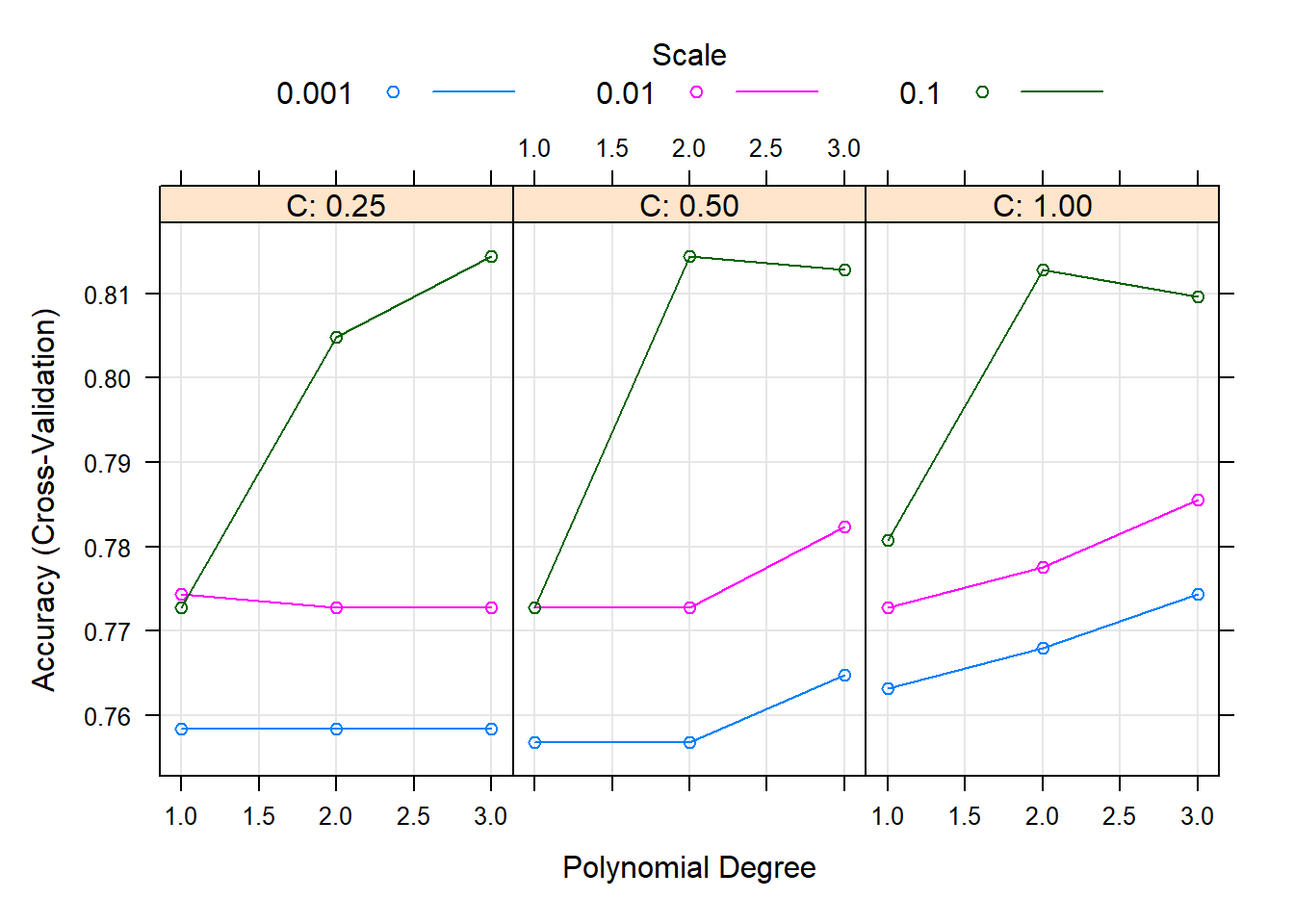
Result! 각 초모수에 대해 랜덤하게 결정된 3개의 값을 조합하여 만든 27(3x3x3)개의 초모수 조합값 (degree, scale, C)에 대한 정확도를 보여주며, (degree = 2, scale = 0.1, C = 0.5)일 때 정확도가 가장 높은 것을 알 수 있다. 따라서 그리드 검색을 통해 찾은 최적의 초모수 조합값 (degree = 2, scale = 0.1, C = 0.5) 근처의 값들을 탐색 범위로 설정하여 훈련을 다시 수행할 수 있다.
customGrid <- expand.grid(degree = 1:3,                  # degree의 탐색 범위
                          scale = seq(0.05, 0.15, 0.05), # scale의 탐색 범위
                          C = seq(0.2, 0.8, 0.1))        # C의 탐색 범위

set.seed(100)                                            # For CV
svm.po.grid.fit <- train(Survived ~ ., data = titanic.trd.Imp,
                         trControl = fitControl,
                         tuneGrid = customGrid,
                         method = "svmPoly",
                         preProc = c("center", "scale")) # Standardization for 예측 변수
svm.po.grid.fit
Support Vector Machines with Polynomial Kernel
625 samples
8 predictor
2 classes: 'no', 'yes'
Pre-processing: centered (8), scaled (8)
Resampling: Cross-Validated (5 fold)
Summary of sample sizes: 500, 500, 500, 500, 500
Resampling results across tuning parameters:
degree scale C Accuracy Kappa
1 0.05 0.2 0.7728 0.5151960
1 0.05 0.3 0.7728 0.5151960
1 0.05 0.4 0.7728 0.5151960
1 0.05 0.5 0.7728 0.5151960
1 0.05 0.6 0.7728 0.5151960
1 0.05 0.7 0.7728 0.5151960
1 0.05 0.8 0.7728 0.5151960
1 0.10 0.2 0.7728 0.5151960
1 0.10 0.3 0.7728 0.5151960
1 0.10 0.4 0.7728 0.5151960
1 0.10 0.5 0.7728 0.5151960
1 0.10 0.6 0.7728 0.5151960
1 0.10 0.7 0.7760 0.5215808
1 0.10 0.8 0.7760 0.5214516
1 0.15 0.2 0.7728 0.5151960
1 0.15 0.3 0.7728 0.5151960
1 0.15 0.4 0.7728 0.5151960
1 0.15 0.5 0.7760 0.5214516
1 0.15 0.6 0.7792 0.5274727
1 0.15 0.7 0.7808 0.5304620
1 0.15 0.8 0.7808 0.5304620
2 0.05 0.2 0.7904 0.5491287
2 0.05 0.3 0.7936 0.5546763
2 0.05 0.4 0.8016 0.5697464
2 0.05 0.5 0.7984 0.5634940
2 0.05 0.6 0.8000 0.5664898
2 0.05 0.7 0.8048 0.5780726
2 0.05 0.8 0.8048 0.5778862
2 0.10 0.2 0.8048 0.5777299
2 0.10 0.3 0.8096 0.5887274
2 0.10 0.4 0.8144 0.5997535
2 0.10 0.5 0.8128 0.5961417
2 0.10 0.6 0.8144 0.5997535
2 0.10 0.7 0.8128 0.5961417
2 0.10 0.8 0.8128 0.5961417
2 0.15 0.2 0.8144 0.5997535
2 0.15 0.3 0.8128 0.5961417
2 0.15 0.4 0.8128 0.5961417
2 0.15 0.5 0.8096 0.5895891
2 0.15 0.6 0.8096 0.5895891
2 0.15 0.7 0.8096 0.5895891
2 0.15 0.8 0.8096 0.5895891
3 0.05 0.2 0.8016 0.5695023
3 0.05 0.3 0.8032 0.5738453
3 0.05 0.4 0.8096 0.5887018
3 0.05 0.5 0.8112 0.5919890
3 0.05 0.6 0.8128 0.5959492
3 0.05 0.7 0.8128 0.5959492
3 0.05 0.8 0.8128 0.5959492
3 0.10 0.2 0.8128 0.5967188
3 0.10 0.3 0.8144 0.6008164
3 0.10 0.4 0.8112 0.5932322
3 0.10 0.5 0.8144 0.6008164
3 0.10 0.6 0.8144 0.6008164
3 0.10 0.7 0.8144 0.6008164
3 0.10 0.8 0.8128 0.5968526
3 0.15 0.2 0.8128 0.5970121
3 0.15 0.3 0.8080 0.5858446
3 0.15 0.4 0.8112 0.5941864
3 0.15 0.5 0.8112 0.5938772
3 0.15 0.6 0.8112 0.5938772
3 0.15 0.7 0.8096 0.5895503
3 0.15 0.8 0.8096 0.5895503
Accuracy was used to select the optimal model using the largest value.
The final values used for the model were degree = 2, scale = 0.15 and C = 0.2.plot(svm.po.grid.fit) # Plot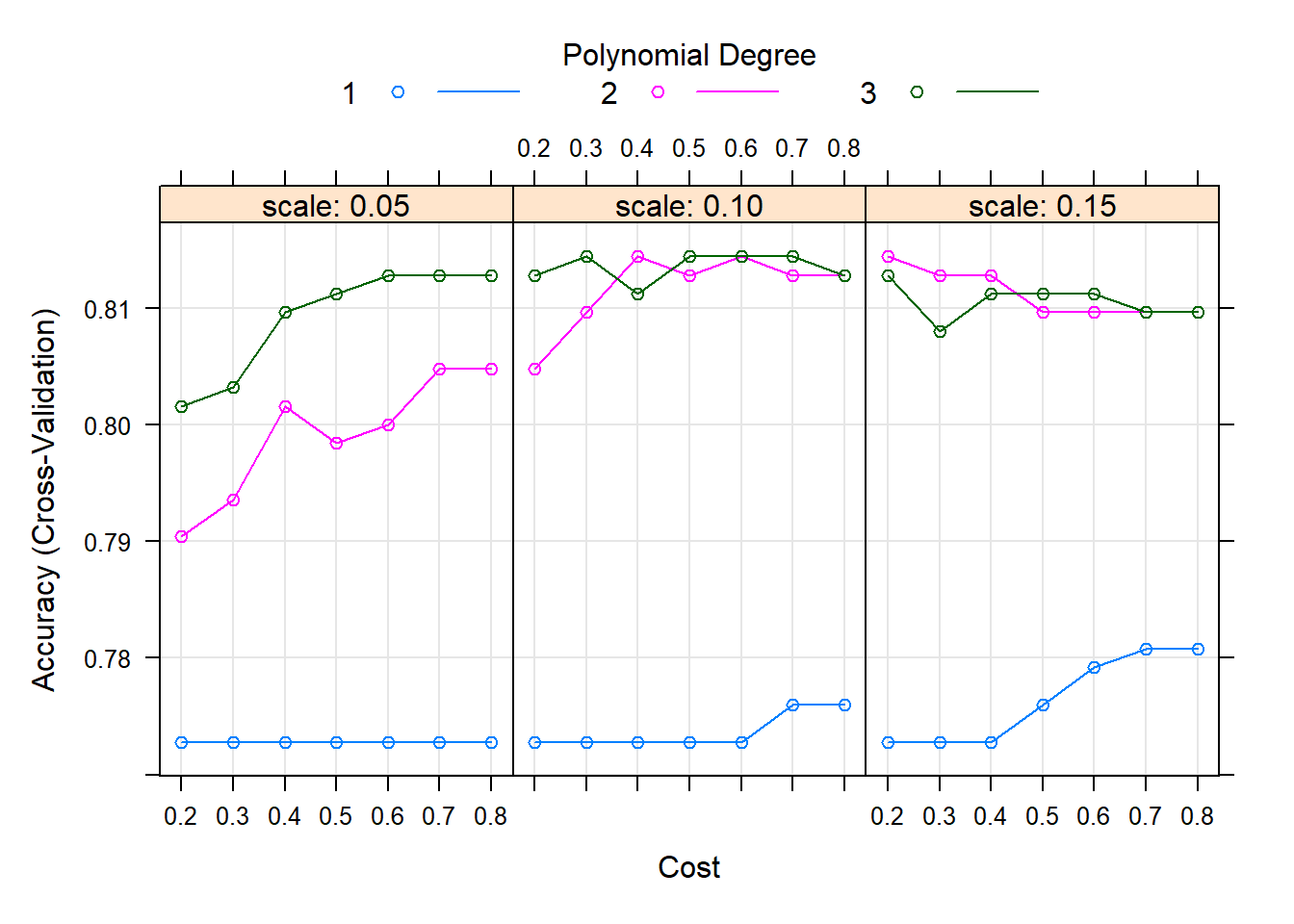
svm.po.grid.fit$bestTune # 최적의 초모수 조합값 degree scale C
36 2 0.15 0.2Result! (degree = 2, scale = 0.15, C = 0.2)일 때 정확도가 가장 높다는 것을 알 수 있으며, (degree = 2, scale = 0.15, C = 0.2)를 가지는 모형을 최적의 훈련된 모형으로 선택한다.
5.7 모형 평가
Caution! 모형 평가를 위해 Test Dataset에 대한 예측 class/확률 이 필요하며, 함수 predict()를 이용하여 생성한다.
# 예측 class 생성
svm.po.pred <- predict(svm.po.grid.fit,
                       newdata = titanic.ted.Imp[,-1])     # Test Dataset including Only 예측 변수

svm.po.pred %>%
  as_tibble
# A tibble: 266 × 1
value
<fct>
1 yes
2 no
3 no
4 yes
5 no
6 no
7 yes
8 no
9 no
10 yes
# ℹ 256 more rows5.7.1 ConfusionMatrix
CM   <- caret::confusionMatrix(svm.po.pred, titanic.ted.Imp$Survived,
                               positive = "yes")         # confusionMatrix(예측 class, 실제 class, positive = "관심 class")
CM
Confusion Matrix and Statistics
Reference
Prediction no yes
no 152 33
yes 12 69
Accuracy : 0.8308
95% CI : (0.7803, 0.8738)
No Information Rate : 0.6165
P-Value [Acc > NIR] : 2.211e-14
Kappa : 0.6277
Mcnemar's Test P-Value : 0.002869
Sensitivity : 0.6765
Specificity : 0.9268
Pos Pred Value : 0.8519
Neg Pred Value : 0.8216
Prevalence : 0.3835
Detection Rate : 0.2594
Detection Prevalence : 0.3045
Balanced Accuracy : 0.8016
'Positive' Class : yes
5.7.2 ROC 곡선
# 예측 확률 생성
test.svm.prob <- predict(svm.po.grid.fit,
                         newdata = titanic.ted.Imp[,-1], # Test Dataset including Only 예측 변수
                         type = "prob")                  # 예측 확률 생성

test.svm.prob %>%
  as_tibble
# A tibble: 266 × 2
no yes
<dbl> <dbl>
1 0.176 0.824
2 0.830 0.170
3 0.816 0.184
4 0.276 0.724
5 0.786 0.214
6 0.884 0.116
7 0.204 0.796
8 0.960 0.0405
9 0.836 0.164
10 0.0320 0.968
# ℹ 256 more rowstest.svm.prob <- test.svm.prob[,2] # "Survived = yes"에 대한 예측 확률
ac <- titanic.ted.Imp$Survived # Test Dataset의 실제 class
pp <- as.numeric(test.svm.prob) # 예측 확률을 수치형으로 변환5.7.2.1 Package “pROC”
pacman::p_load("pROC")

svm.roc  <- roc(ac, pp, plot = T, col = "gray")          # roc(실제 class, 예측 확률)
auc      <- round(auc(svm.roc), 3)
legend("bottomright", legend = auc, bty = "n")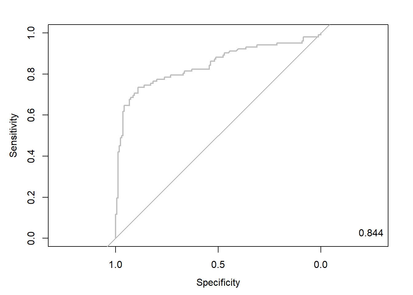
Caution! Package "pROC"를 통해 출력한 ROC 곡선은 다양한 함수를 이용해서 그래프를 수정할 수 있다.
# 함수 plot.roc() 이용
plot.roc(svm.roc,
         col="gray",                                     # Line Color
         print.auc = TRUE,                               # AUC 출력 여부
         print.auc.col = "red",                          # AUC 글씨 색깔
         print.thres = TRUE,                             # Cutoff Value 출력 여부
         print.thres.pch = 19,                           # Cutoff Value를 표시하는 도형 모양
         print.thres.col = "red",                        # Cutoff Value를 표시하는 도형의 색깔
         auc.polygon = TRUE,                             # 곡선 아래 면적에 대한 여부
         auc.polygon.col = "gray90")                     # 곡선 아래 면적의 색깔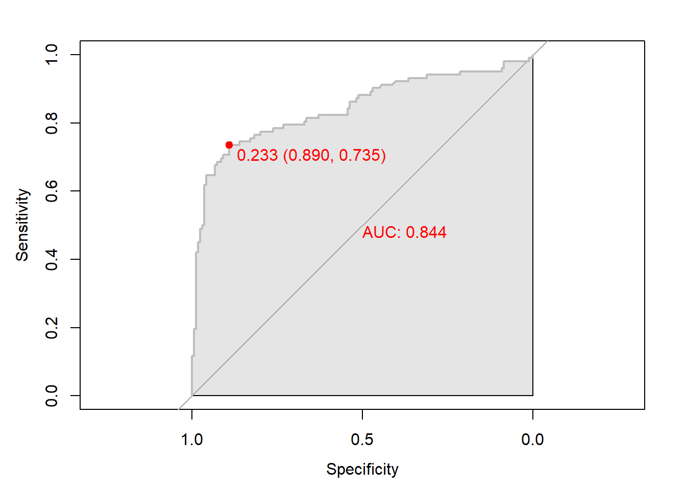
# 함수 ggroc() 이용
ggroc(svm.roc) +
annotate(geom = "text", x = 0.9, y = 1.0,
label = paste("AUC = ", auc),
size = 5,
color="red") +
theme_bw()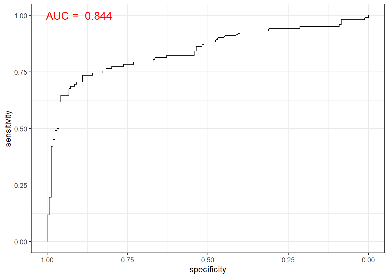
5.7.2.2 Package “Epi”
pacman::p_load("Epi")
# install_version("etm", version = "1.1", repos = "http://cran.us.r-project.org")

ROC(pp, ac, plot = "ROC") # ROC(예측 확률, 실제 class) 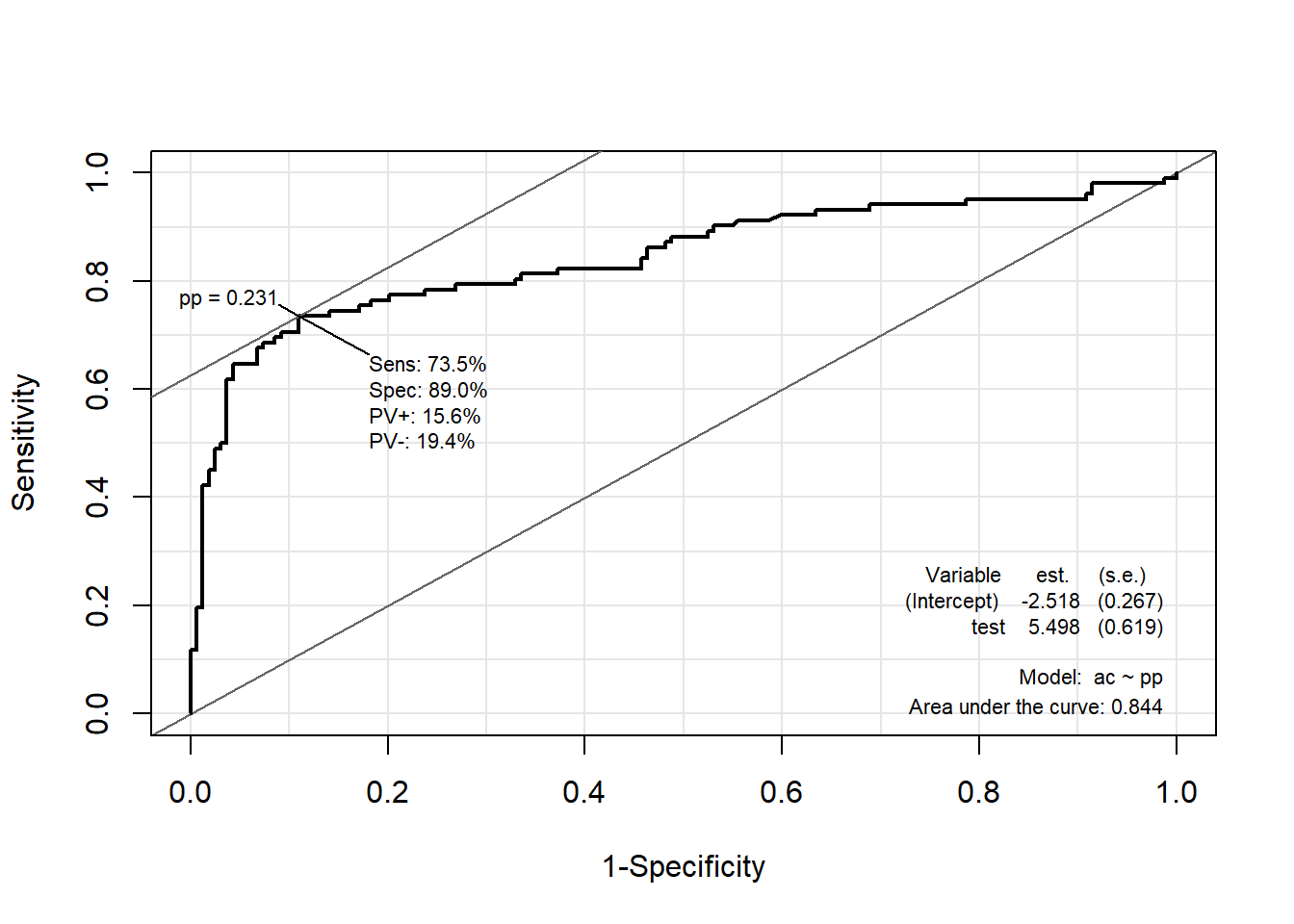
5.7.2.3 Package “ROCR”
pacman::p_load("ROCR")

svm.pred <- prediction(pp, ac)                           # prediction(예측 확률, 실제 class)

svm.perf <- performance(svm.pred, "tpr", "fpr")          # performance(, "민감도", "1-특이도")
plot(svm.perf, col = "gray")                             # ROC Curve

perf.auc   <- performance(svm.pred, "auc")               # AUC
auc        <- attributes(perf.auc)$y.values
legend("bottomright", legend = auc, bty = "n")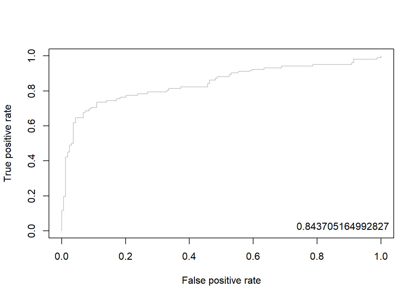
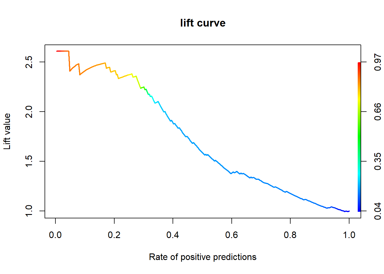
5.7.3 향상 차트
5.7.3.1 Package “ROCR”
svm.perf <- performance(svm.pred, "lift", "rpp")         # Lift Chart
plot(svm.perf, main = "lift curve",
     colorize = T,                                       # Coloring according to cutoff
     lwd = 2)